
How to calculate delta by finite differences? In quantitative finance, Delta measures how sensitive an instrument’s value is to changes in the underlying price.
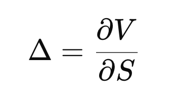
where is the value of the instrument and is the price of the underlying.
In practical terms, Delta answers a simple question:
If the underlying price moves slightly, how much does the price of my instrument move?
A Delta of 0.5 means that a one-unit increase in the underlying price increases the instrument’s value by roughly half a unit. A Delta close to 1 behaves like the underlying itself, while a Delta near 0 barely reacts at all.
This interpretation makes Delta central to both pricing and risk management. Traders use it to hedge exposure, risk systems use it to aggregate sensitivities, and quants use it to reason about how models respond to market moves.
So while Delta is written as a simple derivative, it represents a very concrete financial quantity: exposure to price moves.
1.What are finite differences?
In mathematics, a derivative measures how a quantity changes in the limit of an infinitely small move. In code, however, we never have infinitesimal changes — only finite ones.
A finite difference approximates a derivative by evaluating a function at nearby points and measuring the change.
Formally, the derivative of a function f(x) can be approximated as:
where h is a small but finite step.
Instead of asking how a function behaves at an exact point, finite differences ask a more practical question: what happens if I move the input slightly and recompute the output? This turns abstract calculus into something directly computable using repeated function evaluations.
This idea is at the heart of many numerical methods used in quantitative finance, from Greeks to PDE solvers.
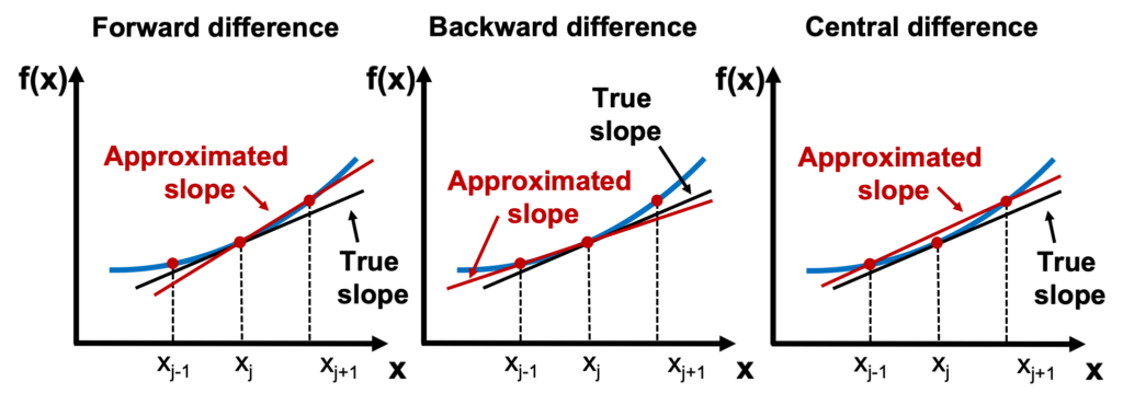
Common Finite Difference Approximations
| Method | Formula | Accuracy | Notes |
|---|---|---|---|
| Forward difference | Simple, biased | ||
| Backward difference | Used near boundaries | ||
| Central difference | Most common in practice |
Here is an illustration of the 3 methods:
2.Apply Finite Differences to Greeks Calculation: The Case of Delta
Delta is defined as the derivative of an instrument’s value with respect to the underlying price. Using finite differences, this derivative can be approximated by bumping the underlying price slightly and re-pricing the instrument. Instead of relying on an analytical expression for Delta, we observe how the price changes in response to a small move in the underlying.
In practice, this means evaluating the pricing function at two nearby prices and measuring the difference:
This central difference approximation is widely used because it is more accurate than one-sided alternatives and symmetric around the current price. It works for any pricing model and any payoff structure, which makes it especially attractive in production systems where models evolve faster than analytical formulas.
Central difference has a second-order truncation error, meaning the approximation error decreases proportionally to as the bump size becomes smaller. In contrast, forward and backward differences only achieve first-order accuracy, with errors proportional to h.
This faster convergence allows central differences to reach a given accuracy with larger bump sizes, which is numerically beneficial in floating-point arithmetic. Larger bumps reduce sensitivity to rounding errors and pricing noise, making the estimate more stable in practice.
In short, central differences strike a better balance between accuracy and numerical robustness. They converge faster, are less biased, and are therefore the default choice for Delta calculations in most quantitative systems.
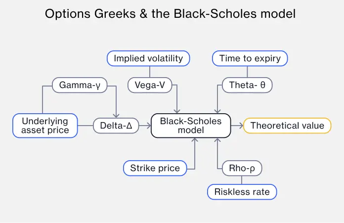
This calculation is usually part of a bigger picture in the Black-Scholes equation giving a theoretical price value:
3. A Practical Example to Illustrate the Calculation
Assume we are pricing a European call option and observe the following prices from our pricing function:
| Underlying Price | Option Price |
|---|---|
| 99.00 | 4.52 |
| 100.00 | 5.00 |
| 101.00 | 5.49 |
We choose a bump size of:
Using the central finite difference formula for Delta:
we plug in the observed values:
A Delta of 0.485 means that, around S=100, a one-unit increase in the underlying price increases the option value by approximately 0.49 units. This aligns with the intuition for a near-the-money call option, whose Delta typically lies between 0.4 and 0.6.
4. An Implementation in C++
In practice, the pricing function used to compute Delta is rarely a simple formula. It is often a reusable component shared across pricing, risk, and valuation workflows. Finite differences work particularly well in this setting because they require no changes to the pricing logic itself.
Consider a simple European call option priced using the Black–Scholes formula. We expose the pricing logic as a callable object and reuse it unchanged to compute Delta.
#include <cmath>

struct BlackScholesCall
{
    double strike;
    double rate;
    double volatility;
    double maturity;

    double operator()(double spot) const
    {
        const double sqrtT = std::sqrt(maturity);
        const double d1 =
            (std::log(spot / strike)
             + (rate + 0.5 * volatility * volatility) * maturity)
            / (volatility * sqrtT);

        const double d2 = d1 - volatility * sqrtT;

        return spot * normal_cdf(d1)
             - strike * std::exp(-rate * maturity) * normal_cdf(d2);
    }
};
The Delta computation itself remains generic:
template<typename Pricer>
double delta(Pricer&& price, double spot, double h)
{
    return (price(spot + h) - price(spot - h)) / (2.0 * h);
}
We can now compute Delta by simply bumping the spot price and reusing the same pricing function:
BlackScholesCall call{100.0, 0.01, 0.20, 1.0};

double spot = 100.0;
double bump = 0.5;

double d = delta(call, spot, bump);
5. Alternative Approaches to Calculate Delta
The appropriate method depends on the pricing model, the complexity of the payoff, and the performance requirements of the system. The table below summarises the most common approaches used in quantitative finance.
| Method | How Delta Is Obtained | Accuracy | Performance | Typical Use Cases |
|---|---|---|---|---|
| Analytical formulas | Closed-form derivative of the pricing formula | Exact (within model) | Very high | Vanilla options, simple models |
| Finite differences | Bump underlying and reprice | Approximate | Medium | General-purpose risk systems |
| PDE-based methods | Local slope on a pricing grid | Approximate | High | Equity and rates models |
| Adjoint (AAD) | Reverse differentiation of the pricer | High | Very high | Large Monte Carlo portfolios |
Finite differences sit at the centre of this spectrum. They are not the most accurate method, nor the fastest, but they are often the most practical. Their simplicity, model-independence, and ease of implementation make them a natural default in many production systems.
Understanding how Delta is computed — and the numerical trade-offs involved — is essential for interpreting risk numbers correctly. A Delta is not just a derivative on paper; it is the result of a numerical procedure, shaped by design choices that matter in practice.