

C++ for Quants
  • Home
  • News
  • Contact
  • About
Author

cppforquants

cppforquant.com
cppforquants

FRM Syllabus
InterviewJobs

The FRM Syllabus: A Guide for C++ Quant Developers

by cppforquants August 13, 2026

The Financial Risk Manager (FRM) certification covers a lot of key concepts: in this article we will talk about the FRM syllabus. For quant developers, it provides a useful framework for understanding the financial models, products, and risk measures that sit behind many real-world systems.

This guide looks at the FRM from a quant developer’s perspective: which topics matter most, how they connect to real development work, and where C++ projects can help turn theory into practical skills.

1. Why Should a Quant Developer Care About the FRM?

Quant developers are usually hired for their programming ability, mathematical background, and understanding of financial markets. In practice, however, writing good C++ or Python is only part of the job. A developer working on pricing, risk, trading, or portfolio systems also needs to understand what the numbers being calculated actually mean.

This is where the Financial Risk Manager (FRM) curriculum can be useful.

The FRM is not a programming qualification, and it will not teach you how to write high-performance C++, design a pricing library, or optimise a Monte Carlo engine. What it does provide is a structured introduction to many of the financial concepts that quant developers encounter in banks, hedge funds, asset managers, and other financial institutions.

Topics such as derivatives, fixed income, probability, statistics, Value at Risk, Expected Shortfall, market risk, credit risk, counterparty exposure, and stress testing are all directly related to systems that quant developers may eventually be asked to build or maintain.

For example, it is one thing to implement a function that calculates VaR. It is another to understand why the calculation is being performed, what assumptions sit behind it, how the result should be interpreted, and where the model can fail.

That domain knowledge becomes particularly valuable when working closely with quantitative analysts, traders, risk managers, and model validation teams.

For a quant developer, the real value of the FRM syllabus is therefore not necessarily the certification itself. It is the financial and risk-management knowledge behind it.

2. FRM 2026 Syllabus at a Glance

How is the FRM exact structured?

FRM Part I

FRM Part I focuses on the fundamental tools used to understand and measure financial risk.
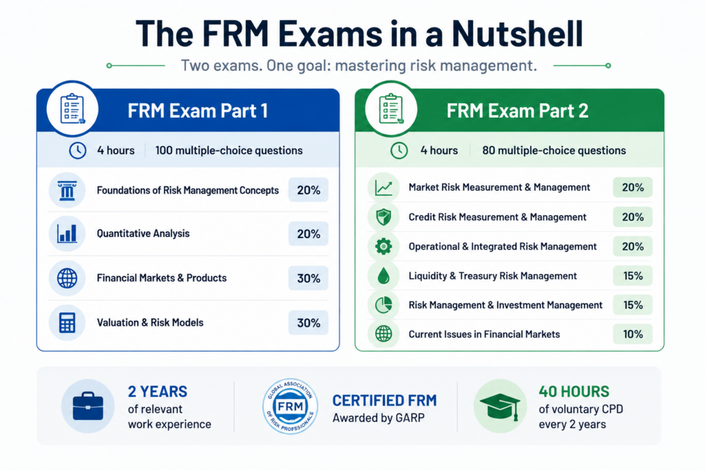
The four main areas are:

  • Foundations of Risk Management
  • Quantitative Analysis
  • Financial Markets and Products
  • Valuation and Risk Models

For quant developers, Part I is especially relevant because it covers many of the concepts that appear in quantitative libraries and risk systems, including:

  • Probability and statistics
  • Regression and time-series analysis
  • Derivatives and fixed-income products
  • Valuation techniques
  • Volatility and correlations
  • Value at Risk (VaR)
  • Expected Shortfall
  • Monte Carlo methods
  • Risk factors and sensitivities

In many ways, Part I provides the mathematical and financial foundations needed to understand what a quantitative system is actually calculating.

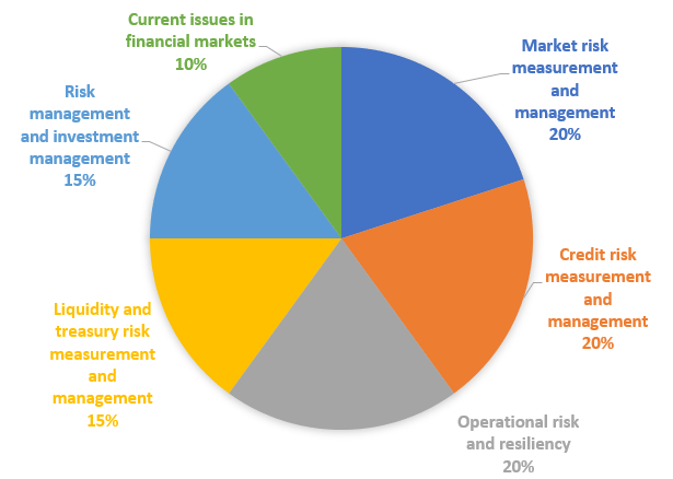
FRM Part II

FRM Part II builds on those foundations and focuses more heavily on applying them to real-world risk management.

The main areas are:

  • Market Risk Measurement and Management
  • Credit Risk Measurement and Management
  • Operational Risk and Resilience
  • Liquidity and Treasury Risk Measurement and Management
  • Risk Management and Investment Management
  • Current Issues in Financial Markets

From a quant developer’s perspective, the most directly relevant topics include:

  • Market risk measurement
  • Scenario analysis
  • Stress testing
  • Value at Risk and Expected Shortfall
  • Credit risk modelling
  • Counterparty exposure
  • Probability of default and loss given default
  • Liquidity risk
  • Portfolio risk
  • Risk aggregation

Part II is closer to the type of work found in production risk infrastructure, where the goal is not simply to value one instrument, but to measure risk across portfolios, counterparties, and changing market conditions.

3. FRM Part I: What Matters to Quant Developers?

FRM Part I is probably the most immediately useful part of the curriculum for a quant developer. It introduces the quantitative tools, financial instruments, valuation techniques, and risk concepts that sit behind many pricing and risk systems.

Some areas have a much stronger connection to quant development than others. Let’s look at each one of the FRM syllabus part 1.

3.1 Quantitative Analysis

Relevance for Quant Developers: ★★★★★

Quantitative Analysis covers much of the mathematical and statistical foundation used throughout quantitative finance. Topics include probability distributions, statistical inference, regression, time-series analysis, volatility estimation, correlation, and simulation methods.

For a quant developer, these concepts appear everywhere.

Typical applications include:

  • Monte Carlo simulation
  • Random number generation
  • Regression models
  • Volatility estimation
  • Correlation and covariance matrices
  • Time-series analysis
  • Statistical model calibration
  • Historical market-data analysis

You may not be responsible for developing every mathematical model yourself, but you will often be responsible for implementing, optimising, testing, or maintaining them.

For example, implementing a Monte Carlo engine requires more than knowing C++. You also need to understand probability distributions, sampling, convergence, correlation, and the statistical meaning of the results.

For this reason, Quantitative Analysis is one of the most valuable FRM areas for a quant developer.

3.2 Financial Markets and Products

Relevance for Quant Developers: ★★★★★

A quant developer also needs to understand the financial instruments represented by the code.

Financial Markets and Products covers areas such as:

  • Futures and forwards
  • Options
  • Swaps
  • Bonds
  • Interest rates
  • Foreign exchange
  • Hedging with derivatives
  • OTC and exchange-traded markets
  • Mortgage-backed securities

These are among the products and market concepts covered within the Part I curriculum.

A class such as:

InterestRateSwap

may look like another C++ object from a software-engineering perspective. From a quantitative-finance perspective, however, you need to understand its legs, cash flows, payment dates, floating-rate resets, discounting, and market-data dependencies.

The same applies to options, futures, bonds, and other instruments.

Understanding the product makes it much easier to:

  • Model trades correctly
  • Design appropriate data structures
  • Understand pricing inputs
  • Interpret Greeks and sensitivities
  • Investigate unexpected results
  • Communicate with traders and quants

This is one of the areas where financial knowledge directly makes you a better quant developer.

3.3 Valuation and Risk Models

Relevance for Quant Developers: ★★★★★

Valuation and Risk Models has perhaps the strongest overlap with traditional quant development.

The area includes topics such as:

  • Value at Risk (VaR)
  • Expected Shortfall
  • Stress testing and scenario analysis
  • Option valuation
  • Fixed-income valuation
  • Hedging
  • Credit risk measures

These are core components of many real-world pricing and risk platforms.

A quant developer working at a bank might encounter systems responsible for:

  • Pricing thousands or millions of trades
  • Calculating portfolio sensitivities
  • Running historical scenarios
  • Calculating VaR or Expected Shortfall
  • Performing stress tests
  • Revaluing portfolios under changing market conditions

This is where mathematical models become software systems.

A formula may fit on a few lines of paper, while its production implementation has to deal with market data, portfolios, numerical methods, performance, concurrency, memory usage, and potentially millions of calculations.

For quant developers interested in pricing engines, risk libraries, derivatives analytics, or front-office systems, this is one of the most relevant parts of the entire FRM curriculum.

4. FRM Part II: What Matters to Quant Developers?

FRM Part II moves away from the foundations and focuses more on how risk is measured and managed across financial institutions.

For quant developers, this is where the curriculum starts to connect more directly with large-scale risk systems, portfolio analytics, counterparty exposure, stress testing, and enterprise infrastructure. Let’s dive into the FRM syllabus part 2.

4.1 Market Risk

Relevance for Quant Developers: ★★★★★

Market Risk is one of the most relevant areas of FRM Part II for quant developers.

It focuses on how changes in market variables such as interest rates, equity prices, foreign exchange rates, credit spreads, and volatility affect portfolios.

Typical topics include:

  • Value at Risk (VaR)
  • Expected Shortfall
  • Stress testing
  • Scenario analysis
  • Backtesting
  • Volatility modelling
  • Correlation
  • Risk-factor modelling
  • Portfolio sensitivities

These concepts appear directly in market-risk platforms and pricing systems.

A quant developer may work on systems that:

  • Generate market scenarios
  • Revalue portfolios
  • Calculate sensitivities
  • Aggregate risk across desks
  • Calculate VaR and Expected Shortfall
  • Run regulatory stress tests
  • Backtest risk models

Market Risk is therefore particularly useful for developers working in banks, trading desks, risk technology teams, and quantitative analytics.

4.2 Credit Risk

Relevance for Quant Developers: ★★★★★

Credit Risk is another highly relevant area, especially for developers working on counterparty risk, XVA, fixed income, or credit derivatives.

Important concepts include:

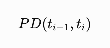
  • Probability of Default (PD)
  • Loss Given Default (LGD)
  • Exposure at Default (EAD)
  • Credit spreads
  • Credit migration
  • Default correlation
  • Counterparty exposure
  • Credit derivatives
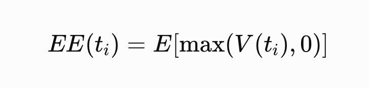
  • Expected exposure
  • Potential Future Exposure (PFE)

These concepts often translate directly into quantitative systems.

For example, a counterparty-risk engine may need to:

  • Simulate future market scenarios
  • Revalue trades at future dates
  • Calculate exposure profiles
  • Apply collateral agreements
  • Aggregate exposure by counterparty
  • Calculate PFE or Expected Exposure
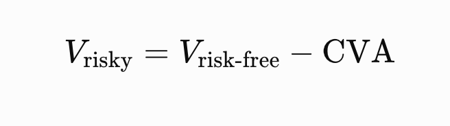
  • Feed results into CVA and other XVA calculations

Credit Risk is especially valuable for quant developers working in large banks, where counterparty-credit and XVA infrastructure can be extremely complex.

4.3 Liquidity and Treasury Risk

Relevance for Quant Developers: ★★★☆☆

Liquidity and Treasury Risk focuses on whether a financial institution can meet its funding and cash-flow obligations under normal and stressed conditions.

Relevant topics include:

  • Funding liquidity
  • Market liquidity
  • Cash-flow forecasting
  • Liquidity stress testing
  • Funding strategies
  • Balance-sheet management
  • Liquidity risk metrics

For quant developers, the relevance depends heavily on the team.

This area is particularly useful for developers working on:

  • Treasury systems
  • Asset and Liability Management (ALM)
  • Funding analytics
  • Liquidity-risk platforms
  • Cash-flow engines
  • Enterprise risk systems

It is less directly relevant to developers working purely on derivatives pricing or low-latency trading systems, but it provides useful knowledge of how banks manage funding and balance-sheet constraints.

4.4 Operational Risk and Resilience

Relevance for Quant Developers: ★★★☆☆

Operational Risk and Resilience is less mathematically focused, but it has more relevance to software engineering than it may initially appear.

Typical areas include:

  • Operational failures
  • Internal controls
  • Cyber and technology risk
  • Model risk
  • Data quality
  • Business continuity
  • System resilience
  • Risk governance

For quant developers working in production environments, many of these issues are very real.

A mathematically correct pricing or risk model is not useful if:

  • The market data is incorrect
  • A batch process fails
  • Results cannot be reproduced
  • A system cannot handle peak workloads
  • Calculations are not properly monitored
  • Model versions are not controlled

This part of the FRM curriculum helps connect quantitative development with the broader operational requirements of running financial systems reliably.

4.5 Risk Management and Investment Management

Relevance for Quant Developers: ★★★☆☆

This area is particularly relevant to developers working in asset management, portfolio analytics, or systematic investment platforms.

Typical concepts include:

  • Portfolio construction
  • Portfolio risk
  • Risk-adjusted performance
  • Factor exposures
  • Asset allocation
  • Performance measurement
  • Investment risk management

For a quant developer, these topics can appear in systems used for:

  • Portfolio optimisation
  • Risk attribution
  • Factor analysis
  • Performance analytics
  • Portfolio construction
  • Asset-allocation models

The relevance is therefore highly role-dependent.

A developer working at an asset manager may use these concepts frequently, while an XVA or derivatives-pricing developer may encounter them much less often.

4.6 Current Issues in Financial Markets

Relevance for Quant Developers: ★★☆☆☆ to ★★★☆☆

Current Issues in Financial Markets focuses on emerging developments and risks affecting the financial industry.

The exact topics change over time, but they may include areas such as:

  • New regulatory developments
  • Changes in market structure
  • Emerging financial risks
  • Technology-related risks
  • Macroeconomic developments
  • New approaches to risk management

For quant developers, the main value is broader industry awareness rather than direct technical knowledge.

Understanding current developments can help explain why banks introduce new models, reporting requirements, data pipelines, or risk calculations.

This section is therefore less likely to help you write better C++ directly, but it can help you understand why the systems around you are changing.

Overall, the most important Part II areas for quant developers are generally Market Risk and Credit Risk, followed by Liquidity, Investment Risk, and Operational Risk depending on the role.

5. FRM vs Building Quant Projects: Where Should You Spend Your Time?

For an aspiring quant developer, the FRM and practical quant projects develop very different skills.

The FRM gives you structured knowledge of financial markets, risk models, derivatives, statistics, and risk management. Building projects teaches you how to turn those concepts into working software.

If your goal is a quant developer role, projects should generally take priority over studying the FRM in isolation.

A hiring manager is more likely to care whether you can:

  • Write clean and efficient C++
  • Implement numerical algorithms correctly
  • Understand financial instruments
  • Work with market data
  • Build pricing and risk models
  • Debug quantitative code
  • Explain the design decisions behind your implementation

This is why the strongest approach is not necessarily to choose between FRM or C++ projects.

Instead, combine them. Learn them and then, implement them. Many topics in the FRM curriculum translate naturally into quant development projects.

For example:

  • Probability and simulation → Build a Monte Carlo simulation framework
  • Options and derivatives → Build a Black-Scholes option pricer
  • Fixed income → Build a yield curve and bond pricing library
  • Value at Risk → Build a historical or Monte Carlo VaR engine
  • Expected Shortfall → Extend your portfolio risk engine
  • Market risk → Build a scenario and stress-testing framework
  • Credit risk → Implement default probability and credit exposure models
  • Counterparty risk → Build a Potential Future Exposure simulator
  • CVA → Build a simple counterparty valuation adjustment engine

This approach gives you both the financial theory and evidence that you can translate it into code.

12. Final Takeaway

The FRM is not a quant development qualification, but parts of its syllabus are highly relevant to the work quant developers do.

Topics such as quantitative analysis, derivatives, valuation, market risk, credit risk, and counterparty exposure all connect directly to pricing libraries, risk engines, portfolio analytics, and other quantitative systems.

The key is to treat the FRM as a source of domain knowledge, not as a substitute for technical skills.

A strong quant developer still needs:

  • Solid C++ and Python
  • Numerical methods
  • Algorithms and data structures
  • Software design
  • Debugging and testing
  • Performance optimisation
  • A good understanding of financial products and models

The most effective approach is to combine both sides.

Use the FRM syllabus to understand the financial concepts, then reinforce that knowledge by implementing them in code.

August 13, 2026 0 comments
Quantlib Architecture
Libraries

QuantLib Architecture: A Tour of Its Core Modules

by cppforquants August 9, 2026

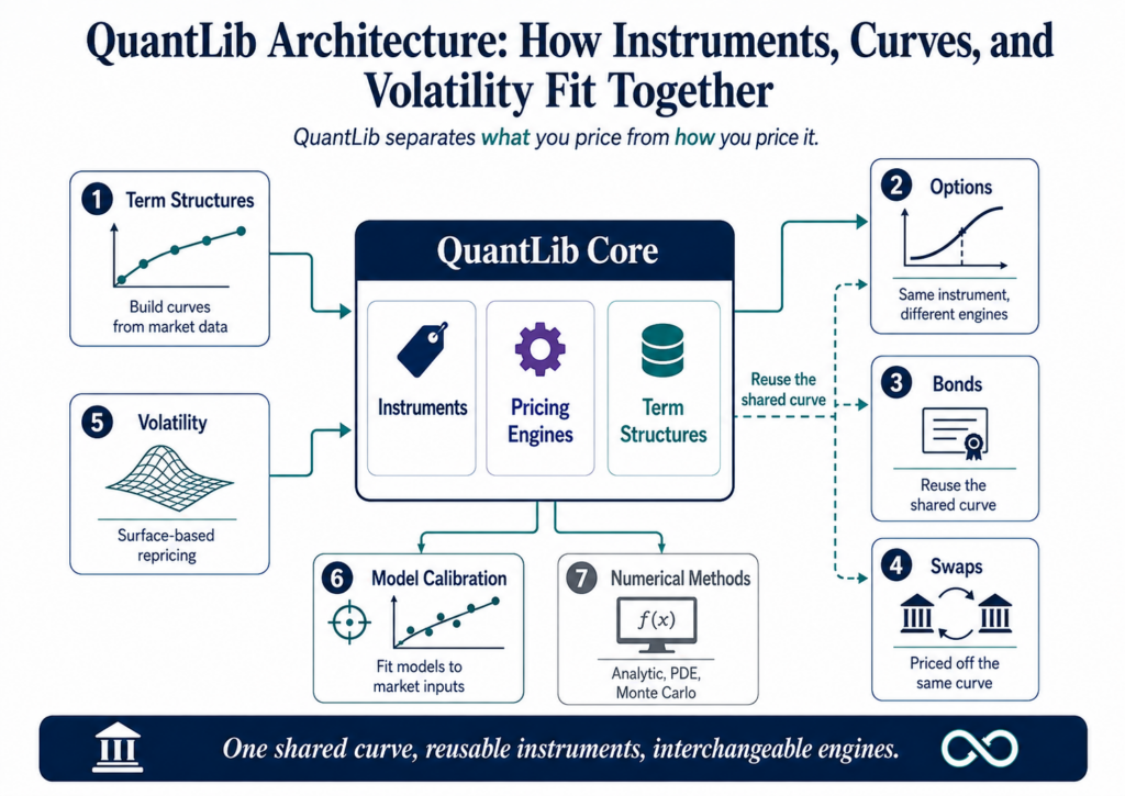
The QuantLib architecture is designed around a clear separation between financial instruments, market data, models, and pricing engines. Instead of tightly coupling each product to a single valuation method, QuantLib lets developers reuse shared term structures, volatility surfaces, and market inputs across options, bonds, swaps, and other instruments.

This modular design is one of the main reasons QuantLib is widely used for quantitative finance and derivatives pricing. In this article, we’ll explore how the core pieces of the QuantLib architecture fit together: from yield curves and volatility structures to pricing engines, numerical methods, and model calibration, and how the same market infrastructure can support multiple valuation workflows.

1. Term Structures

A term structure describes how a financial quantity changes with maturity. In the case of a yield/discount curve, it answers questions such as:

  • What is the discount factor for a cash flow occurring in 3 months?
  • What is the implied zero rate for 5 years?
  • What is the forward rate between years 5 and 7?

The important idea in QuantLib is that a curve is not simply an array of rates. Market data usually gives you only a finite set of quotes—for example, a 3-month deposit rate and swap rates at 1Y, 2Y, 5Y, 10Y, etc. Pricing, however, may require a value at any date.

QuantLib therefore represents the curve as a queryable object. You provide the market instruments and their quotes, and the bootstrapping machinery constructs a YieldTermStructure. You can then ask that object for discount factors, zero rates, or forward rates at arbitrary dates. Interpolation and the conventions used to construct the curve are encapsulated by the term structure rather than being left to every pricing model.

A useful mental model is in the Quantlib architecture framework:

Market quotes → calibration/bootstrapping → queryable term structure → pricing

For example, a discount curve might be bootstrapped from a short-dated deposit followed by a set of interest-rate swaps:

#include <ql/quantlib.hpp>

using namespace QuantLib;

int main() {
    Calendar calendar = TARGET();
    Date today = Date(9, August, 2026);
    Settings::instance().evaluationDate() = today;

    DayCounter dc = Actual365Fixed();

    // Market quotes
    auto depositRate =
        ext::make_shared<SimpleQuote>(0.0250);

    auto swapRate1Y =
        ext::make_shared<SimpleQuote>(0.0270);

    auto swapRate5Y =
        ext::make_shared<SimpleQuote>(0.0320);

    auto swapRate10Y =
        ext::make_shared<SimpleQuote>(0.0350);

    // Convert quotes into RateHelpers.
    auto deposit = ext::make_shared<DepositRateHelper>(
        Handle<Quote>(depositRate),
        Period(3, Months),
        2,
        calendar,
        ModifiedFollowing,
        false,
        Actual360()
    );

    auto swap1Y = ext::make_shared<SwapRateHelper>(
        Handle<Quote>(swapRate1Y),
        Period(1, Years),
        calendar,
        Annual,
        Unadjusted,
        Thirty360(Thirty360::BondBasis),
        Euribor6M()
    );

    auto swap5Y = ext::make_shared<SwapRateHelper>(
        Handle<Quote>(swapRate5Y),
        Period(5, Years),
        calendar,
        Annual,
        Unadjusted,
        Thirty360(Thirty360::BondBasis),
        Euribor6M()
    );

    auto swap10Y = ext::make_shared<SwapRateHelper>(
        Handle<Quote>(swapRate10Y),
        Period(10, Years),
        calendar,
        Annual,
        Unadjusted,
        Thirty360(Thirty360::BondBasis),
        Euribor6M()
    );

    std::vector<ext::shared_ptr<RateHelper>> helpers = {
        deposit, swap1Y, swap5Y, swap10Y
    };

    // Bootstrap the curve from the market instruments.
    auto curve = ext::make_shared<PiecewiseYieldCurve<Discount, LogLinear>>(
        today,
        helpers,
        dc
    );

    // The curve is queryable at arbitrary dates.
    Date fiveYears = calendar.advance(today, Period(5, Years));

    Real discountFactor = curve->discount(fiveYears);
    Rate zeroRate = curve->zeroRate(fiveYears, dc, Continuous).rate();

    std::cout << "5Y discount factor: " << discountFactor << '\n';
    std::cout << "5Y zero rate:       " << zeroRate << '\n';
}

2. Options Pricing

Options pricing is a big big deal in quantitative finance.


In the QuantLib architecture, an Instrument represents the financial contract: its payoff, exercise rules, maturity, and other contractual properties. It does not need to know how its value will be calculated.

The actual valuation is delegated to a PricingEngine.

That separation is useful because the same option can be priced using different numerical methods without changing the definition of the option itself. For example, a European vanilla option can be valued with an analytic Black–Scholes engine, or with a Monte Carlo engine. The VanillaOption remains the same; only the pricing engine changes.

A useful mental model is:

Market data + Instrument → PricingEngine → valuation

Or, more specifically:

What are we pricing? → VanillaOption
How are we pricing it? → PricingEngine

Here’s a simple European call:

#include <ql/quantlib.hpp>

using namespace QuantLib;

int main() {
    Date today(9, August, 2026);
    Settings::instance().evaluationDate() = today;

    Calendar calendar = TARGET();
    DayCounter dc = Actual365Fixed();

    // Market inputs
    Handle<Quote> spot(
        ext::make_shared<SimpleQuote>(100.0)
    );

    Handle<YieldTermStructure> riskFreeCurve(
        ext::make_shared<FlatForward>(
            today, 0.03, dc
        )
    );

    Handle<YieldTermStructure> dividendCurve(
        ext::make_shared<FlatForward>(
            today, 0.00, dc
        )
    );

    Handle<BlackVolTermStructure> volatility(
        ext::make_shared<BlackConstantVol>(
            today, calendar, 0.20, dc
        )
    );

    // Define the option contract.
    auto payoff = ext::make_shared<PlainVanillaPayoff>(
        Option::Call,
        100.0
    );

    Date maturity = calendar.advance(
        today, Period(1, Years)
    );

    auto exercise = ext::make_shared<EuropeanExercise>(
        maturity
    );

    VanillaOption option(payoff, exercise);

    // Choose how to price it.
    auto engine = ext::make_shared<AnalyticEuropeanEngine>(
        Handle<GeneralizedBlackScholesProcess>(
            ext::make_shared<GeneralizedBlackScholesProcess>(
                spot,
                dividendCurve,
                riskFreeCurve,
                volatility
            )
        )
    );

    option.setPricingEngine(engine);

    std::cout << "Option value: "
              << option.NPV()
              << '\n';
}

3. Bonds Pricing

A bond is a sequence of future cash flows: coupons and, eventually, repayment of principal. To value the bond today, those future cash flows need to be discounted back to the valuation date.

In the QuantLib architecture, the FixedRateBond represents the bond contract and its cash flows. It doesn’t itself contain the logic for discounting those cash flows.

The DiscountingBondEngine provides that valuation logic. It takes a YieldTermStructure—such as the curve bootstrapped in the previous section—and uses its discount factors to calculate the present value of the bond’s future cash flows.

So the architecture becomes:

Market quotes → YieldTermStructure → PricingEngine → Instrument value

And importantly, the same curve can be shared by many instruments:

One curve → bonds, swaps, options, and other instruments

Here’s a simple fixed-rate bond using a discount curve:

#include <ql/quantlib.hpp>

using namespace QuantLib;

int main() {
    Date today(9, August, 2026);
    Settings::instance().evaluationDate() = today;

    Calendar calendar = TARGET();
    DayCounter dc = ActualActual(ActualActual::Bond);

    // In practice, this would be the bootstrapped curve
    // from Section 1.
    Handle<YieldTermStructure> discountCurve(
        ext::make_shared<FlatForward>(
            today,
            0.03,
            dc
        )
    );

    // Define the bond.
    Natural settlementDays = 2;
    Date issueDate = today;
    Date maturityDate = calendar.advance(
        issueDate, Period(5, Years)
    );

    Schedule schedule(
        issueDate,
        maturityDate,
        Period(Annual),
        calendar,
        Unadjusted,
        Unadjusted,
        DateGeneration::Backward,
        false
    );

    Real couponRate = 0.04;

    FixedRateBond bond(
        settlementDays,
        100.0,                  // face value
        schedule,
        std::vector<Rate>{couponRate},
        dc
    );

    // Tell the bond how it should be valued.
    auto engine =
        ext::make_shared<DiscountingBondEngine>(
            discountCurve
        );

    bond.setPricingEngine(engine);

    std::cout << "Bond NPV: "
              << bond.NPV()
              << '\n';

    std::cout << "Clean price: "
              << bond.cleanPrice()
              << '\n';

    std::cout << "Dirty price: "
              << bond.dirtyPrice()
              << '\n';
}

Another example in this video:

4. Interest Rate Swaps

An interest rate swap exchanges two streams of interest payments, typically a fixed rate against a floating rate. In a vanilla fixed-for-floating swap, one party pays a fixed rate while receiving a floating rate, usually based on an index such as 6-month Euribor.

From a pricing perspective, the swap is essentially a comparison of two legs:

  • the fixed leg, whose future payments are known from the swap’s fixed rate;
  • the floating leg, whose future payments depend on the evolution of interest rates.

QuantLib architecture represents the contract with VanillaSwap. The actual valuation is delegated to a pricing engine, such as DiscountingSwapEngine.

This is where the term structure from Section 1 becomes particularly useful. The same YieldTermStructure that was bootstrapped from market quotes can be passed into the swap’s pricing engine to discount the swap’s future cash flows.

A useful mental model is:

Curve → discounting and forward-rate information → swap valuation

Or, across the sections you’ve built so far:

Market quotes → YieldTermStructure → financial instrument → PricingEngine → NPV

Here is a simple vanilla swap:

#include <ql/quantlib.hpp>

using namespace QuantLib;

int main() {
    Date today(9, August, 2026);
    Settings::instance().evaluationDate() = today;

    Calendar calendar = TARGET();
    DayCounter dc = Actual365Fixed();

    // In practice, reuse the bootstrapped curve
    // from Section 1.
    Handle<YieldTermStructure> curve(
        ext::make_shared<FlatForward>(
            today,
            0.03,
            dc
        )
    );

    // Swap terms
    Date startDate = calendar.advance(
        today, Period(2, Days)
    );

    Date maturityDate = calendar.advance(
        startDate, Period(5, Years)
    );

    Schedule fixedSchedule(
        startDate,
        maturityDate,
        Period(Annual),
        calendar,
        ModifiedFollowing,
        ModifiedFollowing,
        DateGeneration::Forward,
        false
    );

    Schedule floatingSchedule(
        startDate,
        maturityDate,
        Period(Semiannual),
        calendar,
        ModifiedFollowing,
        ModifiedFollowing,
        DateGeneration::Forward,
        false
    );

    // Build the vanilla fixed-for-floating swap.
    Rate fixedRate = 0.0325;

    VanillaSwap swap(
        VanillaSwap::Payer,       // pay fixed, receive floating
        1'000'000.0,              // notional
        fixedSchedule,
        fixedRate,
        dc,
        floatingSchedule,
        Euribor6M(curve),
        0.0,                       // spread
        Actual360()
    );

    // Use the same curve to discount the swap.
    auto engine =
        ext::make_shared<DiscountingSwapEngine>(curve);

    swap.setPricingEngine(engine);

    std::cout << "Swap NPV: "
              << swap.NPV()
              << '\n';

    std::cout << "Fair fixed rate: "
              << swap.fairRate()
              << '\n';
}

5. Volatility Surface

A volatility surface captures this two-dimensional relationship and it can often look like a smile.

In QuantLib architecture, BlackVarianceSurface represents this market information as a queryable object. Instead of asking for “the volatility,” a pricing engine can effectively ask:

What volatility should I use for this particular maturity and strike?

That makes it conceptually similar to the term structure from Section 1: rather than storing a handful of market observations as disconnected numbers, QuantLib turns them into a reusable object that can be queried by pricing models.

The architecture becomes:

Market volatility quotes → BlackVarianceSurface → PricingEngine → option value

And because the VanillaOption from Section 2 doesn’t change, we can simply replace its flat-volatility input with the surface and reprice it.

Here’s a compact example using a small grid of implied volatilities:

#include <ql/quantlib.hpp>

using namespace QuantLib;

int main() {
    Date today(9, August, 2026);
    Settings::instance().evaluationDate() = today;

    Calendar calendar = TARGET();
    DayCounter dc = Actual365Fixed();

    // Underlying and curves from Section 2.
    Handle<Quote> spot(
        ext::make_shared<SimpleQuote>(100.0)
    );

    Handle<YieldTermStructure> riskFreeCurve(
        ext::make_shared<FlatForward>(
            today, 0.03, dc
        )
    );

    Handle<YieldTermStructure> dividendCurve(
        ext::make_shared<FlatForward>(
            today, 0.00, dc
        )
    );

    // Maturities represented by the surface.
    std::vector<Date> dates = {
        calendar.advance(today, Period(6, Months)),
        calendar.advance(today, Period(1, Years)),
        calendar.advance(today, Period(2, Years))
    };

    // Strikes represented by the surface.
    std::vector<Real> strikes = {
        90.0, 100.0, 110.0
    };

    // Implied volatility matrix:
    //
    //             90%     100%     110%
    //  6M        22%      20%      21%
    //  1Y        21%      19%      20%
    //  2Y        20%      18%      19%
    //
    Matrix vols(dates.size(), strikes.size());

    vols[0][0] = 0.22;
    vols[0][1] = 0.20;
    vols[0][2] = 0.21;

    vols[1][0] = 0.21;
    vols[1][1] = 0.19;
    vols[1][2] = 0.20;

    vols[2][0] = 0.20;
    vols[2][1] = 0.18;
    vols[2][2] = 0.19;

    // Build the volatility surface.
    auto surface = ext::make_shared<BlackVarianceSurface>(
        today,
        calendar,
        dates,
        strikes,
        vols,
        dc
    );

    Handle<BlackVolTermStructure> volatility(surface);

    // The same option from Section 2.
    auto payoff =
        ext::make_shared<PlainVanillaPayoff>(
            Option::Call,
            100.0
        );

    Date maturity = calendar.advance(
        today, Period(1, Years)
    );

    auto exercise =
        ext::make_shared<EuropeanExercise>(maturity);

    VanillaOption option(payoff, exercise);

    auto process =
        ext::make_shared<GeneralizedBlackScholesProcess>(
            spot,
            dividendCurve,
            riskFreeCurve,
            volatility
        );

    auto engine =
        ext::make_shared<AnalyticEuropeanEngine>(process);

    option.setPricingEngine(engine);

    std::cout << "Option value with volatility surface: "
              << option.NPV()
              << '\n';
}

6. Model Calibration

Calibration is the process of choosing a model’s parameters so that the model reproduces prices or quotes observed in the market.

For example, suppose we want to use the Hull–White short-rate model. The model has parameters controlling the behaviour of interest rates, such as mean reversion and volatility. Those parameters aren’t arbitrary: we want to choose them so that the model is consistent with instruments that are actually traded in the market.

Conceptually:

Market quotes → instruments → model → calibration → model parameters

This is different from bootstrapping a curve.

A curve bootstrapping process asks:

What discount factors are consistent with these market instruments?

Calibration asks:

What model parameters make this model reproduce the prices of these market instruments?

Here is a deliberately compact example:

#include <ql/quantlib.hpp>

using namespace QuantLib;

int main() {
    Date today(9, August, 2026);
    Settings::instance().evaluationDate() = today;

    Calendar calendar = TARGET();
    DayCounter dc = Actual365Fixed();

    // Reuse the curve built in Section 1.
    Handle<YieldTermStructure> curve(
        ext::make_shared<FlatForward>(
            today, 0.03, dc
        )
    );

    // Hull-White model.
    auto model = ext::make_shared<HullWhite>(
        curve,
        0.10,   // mean reversion
        0.01    // short-rate volatility
    );

    // Market instruments used for calibration.
    std::vector<ext::shared_ptr<CalibrationHelper>> helpers;

    std::vector<Period> maturities = {
        Period(1, Years),
        Period(2, Years),
        Period(5, Years),
        Period(10, Years)
    };

    std::vector<Volatility> marketVols = {
        0.20,
        0.21,
        0.23,
        0.25
    };

    for (Size i = 0; i < maturities.size(); ++i) {
        auto helper =
            ext::make_shared<SwaptionHelper>(
                maturities[i],
                Period(5, Years),
                Handle<Quote>(
                    ext::make_shared<SimpleQuote>(
                        marketVols[i]
                    )
                ),
                Euribor6M(curve),
                Period(1, Years),
                Thirty360(Thirty360::BondBasis),
                dc,
                curve
            );

        helpers.push_back(helper);
    }

    // Give every calibration instrument the model.
    auto engine =
        ext::make_shared<TreeSwaptionEngine>(
            model,
            50
        );

    for (auto& helper : helpers)
        helper->setPricingEngine(engine);

    // Optimize the model parameters so model prices
    // reproduce the market instruments.
    model->calibrate(
        helpers,
        LevenbergMarquardt(),
        EndCriteria(
            1000,    // max iterations
            100,     // max stationary state
            1e-8,    // root epsilon
            1e-8,    // function epsilon
            1e-8     // gradient norm epsilon
        )
    );

    std::cout << "Mean reversion: "
              << model->a()
              << '\n';

    std::cout << "Volatility: "
              << model->sigma()
              << '\n';
}

August 9, 2026 0 comments
Order Book C++
Data StructuresInterviewPerformance

Data Structures for Order Book: std::map, std::unordered_map, or std::vector?

by cppforquants July 12, 2026

Ask a C++ developer to design a limit order book, and you will almost always get the same answer: std::map<Price, Level>. It is the answer every tutorial gives, the answer that passes the coding screen, and the answer that feels obviously right: an order book is a collection of price levels that must stay sorted, and std::map is the sorted container. Case closed.

Except that if you look at how production trading systems are actually built, you will struggle to find a red-black tree anywhere near the hot path. The container that “obviously” fits the problem is quietly absent from the systems where the problem matters most.

This article explains why, by putting three candidates through the same test: std::unordered_map, std::map, and — the one nobody suggests in interviews — std::vector.


1.Refresher on std::map, std::unordered_map and std::vectors

What are maps?

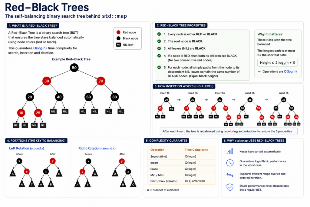
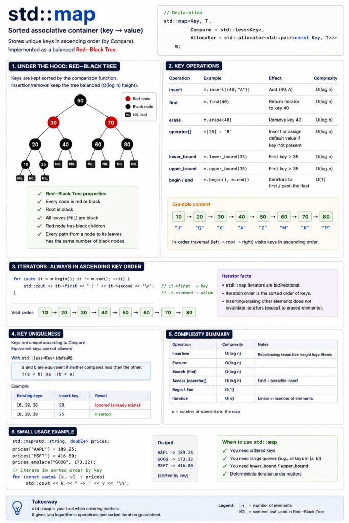
A std::map is a sorted associative container storing key-value pairs with unique keys, typically implemented as a red-black tree.

Lookups, insertions, and deletions are all O(log n), and iterating gives you elements in key order.

A good summary video:

What are unordered maps?

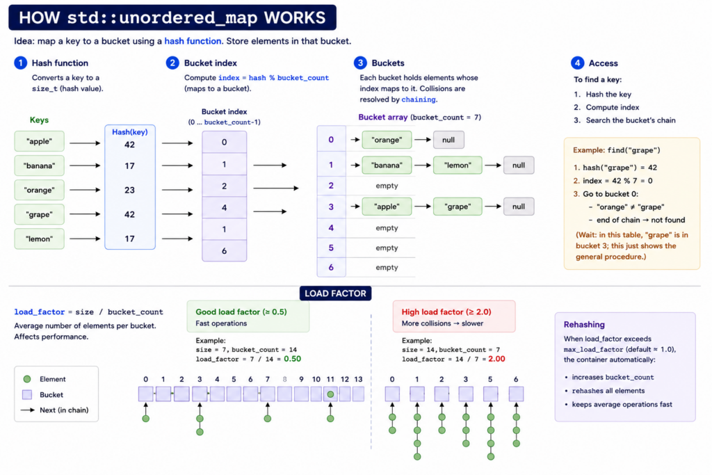
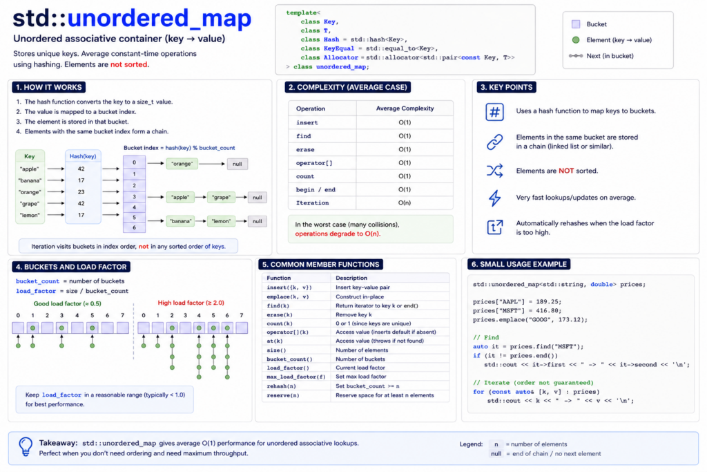
A std::unordered_map is a hash table storing key-value pairs with unique keys but no ordering guarantee.

Average O(1) lookup, insert, and erase, degrading to O(n) in the worst case (hash collisions).

The trade-offs: it needs a hash function for the key type, iteration order is unspecified, and the node-based bucket implementation means pointer chasing that can hurt cache performance — which is why HFT code often reaches for open-addressing alternatives like absl::flat_hash_map.

What are vectors?


std::vector is C++’s dynamic array: it stores elements in contiguous memory, gives fast indexed access, and automatically grows when you add more elements.

How to use them to create an order book? But, by the way, what’s an order book?


2. Refresher on order books

An order book is the mechanism that allows a market to match buyers and sellers.

A trader can send:

Buy 100 shares at 99.98
Sell 200 shares at 100.02
Buy 50 shares at market
Cancel order #123
Modify order #456

The exchange maintains the book and decides what happens next.

An order book is the live list of buyers and sellers for a financial instrument.

At first, it is often shown as a table:

Bid SizeBid PriceAsk PriceAsk Size
500 99.98 100.02 300
1,200 99.97 100.03 700
800 99.96 100.04 1,500

The bid side represents buyers.
The ask side represents sellers.

Here, “size” means quantity.

So:

500 at 99.98 means buyers want to buy 500 shares at 99.98.
300 at 100.02 means sellers want to sell 300 shares at 100.02.

Each row is also called a price level.

Level 1 is the best available price on each side:

Level 1 bid = 99.98 x 500
Level 1 ask = 100.02 x 300

Level 2 is the next best price:

Level 2 bid = 99.97 x 1,200
Level 2 ask = 100.03 x 700

Level 3 is the next one after that:

Level 3 bid = 99.96 x 800
Level 3 ask = 100.04 x 1,500

A more natural way to visualize the book is vertically:

            ASK SIDE

Level 3     100.04 x 1,500
Level 2     100.03 x 700
Level 1     100.02 x 300     <- best ask

            spread = 0.04

Level 1      99.98 x 500     <- best bid
Level 2      99.97 x 1,200
Level 3      99.96 x 800

            BID SIDE

The best bid is the highest price someone is willing to buy at.
The best ask is the lowest price someone is willing to sell at.

3. Model an Order Book in C++: Various Attempts

Attempt 1: hash the price levels with std::unordered_map

The message flow suggests an obvious first design. Cancels dominate, and cancels are lookups — so we optimize for lookup. A hash map from price to level gives us O(1) access to any level, and std::unordered_map is sitting right there in the standard library:

cpp

std::unordered_map<Price, Level> bids_;
std::unordered_map<Price, Level> asks_;

Adds are O(1). Cancels are O(1). Modifies are O(1). On paper we’ve made the dominant operations constant-time, and for a few minutes this feels like a solved problem.

Then we implement best_bid().

There is no “first element” in a hash map. Hashing deliberately destroys ordering — that’s what makes it fast — so the only way to find the highest bid is to scan every populated level. The book’s single most frequent query, the one strategy code calls on effectively every tick, has become O(n) over the entire side. Depth walks are worse: there’s no notion of “the next level down” at all; we’d re-scan or sort on demand.

We didn’t build a slow order book. We built something that structurally isn’t an order book. An order book’s defining property is that its levels are ordered — it’s in the name — and we chose the one container whose entire design premise is discarding order. The lookup speed was real, but we optimized the operation that was never going to be the bottleneck and broke the one that defines the product.

Attempt 2: the tree with std::map

So ordering is non-negotiable. The standard library’s ordered associative container is std::map, a red-black tree, and it fixes everything the hash map broke:

std::map<Price, Level, std::greater<Price>> bids_;  // begin() is best bid
std::map<Price, Level> asks_;                        // begin() is best ask

Best bid is bids_.begin() — O(1). Depth walks are in-order traversal. Adds, cancels, and modifies are O(log n), and with a few hundred populated levels, log n is under ten comparisons. This is the textbook answer, it’s correct, and it’s what most order book implementations you’ll find online actually use.

Now replay a day of market data through it and watch what the hardware does.

A full implementation of that version that would make you pass the quant interview in C++ has been proposed in our first article on order books:

using OrderId   = uint64_t;
using Qty       = int64_t;        // signed for partial fills math
using Px       = int64_t;         // price in ticks
enum Side { Buy, Sell };

struct Order {
  OrderId id;
  Side side;
  Px price;
  Qty qty;            // remaining
  uint64_t ts;        // exchange/seq time for tie-breaks
  // intrusive list pointers for O(1) erase
  Order* prev = nullptr;
  Order* next = nullptr;
};

struct Level {
  Px price;
  Order* head = nullptr;
  Order* tail = nullptr;
  inline void push_back(Order* o);
  inline void erase(Order* o);
  bool empty() const { return head == nullptr; }
};

// price → level; bids need descending, asks ascending
using BookSide = std::map<Px, Level, std::greater<Px>>;     // bids
using BookSideAsk = std::map<Px, Level, std::less<Px>>;     // asks

struct OrderBook {
  BookSide bids;
  BookSideAsk asks;
  std::unordered_map<OrderId, Order*> by_id;  // direct handle for cancel/replace

  // API
  void add_limit(OrderId id, Side side, Px px, Qty qty, uint64_t ts);
  void cancel(OrderId id);
  void replace(OrderId id, Px new_px, Qty new_qty, uint64_t ts); // cancel+add semantics
  void match_market(Side side, Qty qty);
  // helpers
  Level& level(BookSide& s, Px px);
  Level& level(BookSideAsk& s, Px px);
};

Attempt 3: keep it sorted, make it contiguous

If pointer chasing is the disease, contiguity is the cure. A sorted std::vector<Level> with binary search keeps the ordering guarantee but lays every level out in a single flat allocation:

cpp

std::vector<Level> bids_;  // sorted; back() is best bid

Lookup is std::lower_bound — still O(log n) comparisons, but now the search touches a handful of cache lines in one array instead of five scattered heap nodes, and the hardware prefetcher can see where we’re going. Best bid is back(). Insertion of a new level requires shifting elements — O(n) in theory — but here the workload rescues us: adds cluster near the touch, so if the vector is sorted with the best price at the back, the memmove is almost always a few elements. In practice this structure embarrasses the tree on a realistic feed.

And yet, benchmark it honestly and there’s a residue we can’t scrub out. Every operation still begins with a search — a binary search is a series of dependent loads, each one’s address unknown until the previous compare resolves, so the pipeline stalls on each step. We’ve made searching cheap. We haven’t asked whether we need to search at all.

Attempt 4: stop searching

Every structure so far has treated the price as an opaque key — something to hash, compare, or binary-search for. But a price in a limit order book is none of those things. Exchanges don’t accept arbitrary prices: every instrument trades on a fixed grid, an integer number of ticks. Two consecutive price levels don’t just happen to be close — they differ by exactly one tick, always. That’s not a statistical tendency we can exploit; it’s a hard constraint the venue enforces on every order.

Once you see prices as grid positions rather than keys, the search problem dissolves. If we know the tick size and pick an anchor price for index zero, then the level for any price isn’t something we find — it’s something we compute.

index = (price − anchor) / tick

One subtraction, one division by a constant, one indexed load into a flat array. No hash function, no comparisons, no dependent loads waiting on the previous step to resolve. The lookup that cost the tree five scattered pointer dereferences and cost the sorted vector a pipeline-stalling binary search is now cheaper than either structure’s first step.

4. A Proposition of Implementation for Attempt 4

In the approach we’re presenting, prices are ticks on a fixed grid, so the book is a flat array of price levels where a price is converted to an index by one subtraction — no hashing, no tree, no search — with a cached best index and each level holding a FIFO of pool-allocated orders linked intrusively.

Adds, cancels, and executions each cost an arithmetic index or an O(1) ID lookup plus an O(1) unlink, touching two or three cache lines and zero heap allocations on the hot path.

Let’s start with an order_book.hpp:

// order_book.hpp — tick-indexed limit order book
//
// Design (see article): contiguous array of price levels indexed by tick
// offset, intrusive doubly-linked FIFO per level, pre-allocated order pool,
// open-addressing map for OrderId -> Order*. Zero heap allocation on the
// hot path after construction.
//
// Conventions:
//   - Price is an integer number of ticks (scale at the feed decoder).
//   - OrderId 0 and ~0 are reserved (empty / tombstone sentinels in IdMap).

#pragma once

#include <cassert>
#include <cstddef>
#include <cstdint>
#include <vector>

using Price   = std::int64_t;
using Qty     = std::int64_t;
using OrderId = std::uint64_t;

enum class Side : std::uint8_t { Bid, Ask };

// ---------------------------------------------------------------------------
// Order: 64 bytes, cache-line aligned. prev/next are intrusive — the order
// *is* its own list node, so joining/leaving a level allocates nothing.
// ---------------------------------------------------------------------------
struct alignas(64) Order {
    OrderId id;
    Qty     qty;
    Price   price;
    Side    side;
    Order*  prev;
    Order*  next;
};
static_assert(sizeof(Order) == 64, "one order per cache line");

// ---------------------------------------------------------------------------
// OrderPool: all orders live in one contiguous slab allocated at startup.
// alloc/release are a free-list push/pop — no new/delete on the hot path.
// ---------------------------------------------------------------------------
class OrderPool {
public:
    explicit OrderPool(std::size_t capacity) : slots_(capacity) {
        free_.reserve(capacity);
        for (std::size_t i = capacity; i-- > 0;)
            free_.push_back(&slots_[i]);
    }

    Order* alloc() {
        assert(!free_.empty() && "pool exhausted — size it to the session");
        Order* o = free_.back();
        free_.pop_back();
        return o;
    }

    void release(Order* o) { free_.push_back(o); }

private:
    std::vector<Order>  slots_;
    std::vector<Order*> free_;
};

// ---------------------------------------------------------------------------
// Level: FIFO queue of resting orders at one price. head is oldest (first to
// fill), tail is where adds append — price-time priority falls out of the
// list order. total_qty is maintained incrementally so top-of-book snapshots
// never walk the list.
// ---------------------------------------------------------------------------
struct Level {
    Order* head      = nullptr;
    Order* tail      = nullptr;
    Qty    total_qty = 0;

    bool empty() const { return head == nullptr; }

    void push_back(Order* o) {
        o->prev = tail;
        o->next = nullptr;
        if (tail) tail->next = o; else head = o;
        tail = o;
        total_qty += o->qty;
    }

    // O(1) given the order pointer — no search. This is why cancels, the
    // dominant message type, stay cheap.
    void unlink(Order* o) {
        if (o->prev) o->prev->next = o->next; else head = o->next;
        if (o->next) o->next->prev = o->prev; else tail = o->prev;
        total_qty -= o->qty;
    }
};

// ---------------------------------------------------------------------------
// BookSide: the tick-indexed array. Price -> level is one subtraction and
// one indexed load; no hashing, no comparisons, no pointer chasing.
// best_ caches the top of book; when the top level empties we scan linearly
// toward the interior — adjacent prices are adjacent cache lines, and the
// next populated level is almost always within a few ticks.
// ---------------------------------------------------------------------------
template <bool IsBid>
class BookSide {
public:
    static constexpr std::size_t kLevels = std::size_t{1} << 16;
    static constexpr std::size_t kNone   = ~std::size_t{0};

    explicit BookSide(Price anchor)
        : levels_(kLevels), anchor_(anchor) {}

    void add(Order* o) {
        const std::size_t idx = index(o->price);
        levels_[idx].push_back(o);
        if (best_ == kNone || better(idx, best_)) best_ = idx;
    }

    void remove(Order* o) {
        const std::size_t idx = index(o->price);
        levels_[idx].unlink(o);
        if (idx == best_ && levels_[idx].empty()) advance_best();
    }

    void reduce(Order* o, Qty by) {
        o->qty -= by;
        levels_[index(o->price)].total_qty -= by;
    }

    bool  empty()      const { return best_ == kNone; }
    Price best_price() const { return anchor_ + static_cast<Price>(best_); }
    Qty   best_qty()   const { return levels_[best_].total_qty; }
    const Order* best_order() const { return levels_[best_].head; }

private:
    std::size_t index(Price p) const {
        assert(p >= anchor_ &&
               static_cast<std::size_t>(p - anchor_) < kLevels &&
               "price outside book range — re-anchor on the slow path");
        return static_cast<std::size_t>(p - anchor_);
    }

    static bool better(std::size_t a, std::size_t b) {
        if constexpr (IsBid) return a > b;   // best bid = highest price
        else                 return a < b;   // best ask = lowest price
    }

    void advance_best() {
        if constexpr (IsBid) {
            while (best_ != 0) {
                --best_;
                if (!levels_[best_].empty()) return;
            }
        } else {
            while (best_ + 1 < kLevels) {
                ++best_;
                if (!levels_[best_].empty()) return;
            }
        }
        best_ = kNone;   // side is empty
    }

    std::vector<Level> levels_;   // one flat allocation, made once
    Price              anchor_;   // price at index 0
    std::size_t        best_ = kNone;
};

// ---------------------------------------------------------------------------
// IdMap: OrderId -> Order*, open addressing with linear probing. Flat slot
// array — one hash, then a short contiguous probe. Sized 2x expected load
// at construction; erases leave tombstones (fine for a trading session,
// rebuild between sessions if reusing).
// ---------------------------------------------------------------------------
// ---------------------------------------------------------------------------
// IdMap: OrderId -> Order*, open addressing with linear probing. Flat slot
// array — one hash, then a short contiguous probe. Sized 2x expected load
// at construction; erases leave tombstones (fine for a trading session,
// rebuild between sessions if reusing).
// ---------------------------------------------------------------------------
class IdMap {
public:
    explicit IdMap(std::size_t expected) {
        std::size_t cap = 1;
        while (cap < expected * 2) cap <<= 1;
        slots_.assign(cap, Slot{kEmpty, nullptr});
        mask_ = cap - 1;
    }

    void insert(OrderId id, Order* o) {
        std::size_t i = hash(id) & mask_;
        while (slots_[i].key != kEmpty && slots_[i].key != kTomb)
            i = (i + 1) & mask_;
        slots_[i] = Slot{id, o};
    }

    Order* find(OrderId id) const {
        std::size_t i = hash(id) & mask_;
        while (slots_[i].key != kEmpty) {
            if (slots_[i].key == id) return slots_[i].val;
            i = (i + 1) & mask_;
        }
        return nullptr;
    }

    void erase(OrderId id) {
        std::size_t i = hash(id) & mask_;
        while (slots_[i].key != kEmpty) {
            if (slots_[i].key == id) {
                slots_[i].key = kTomb;
                slots_[i].val = nullptr;
                return;
            }
            i = (i + 1) & mask_;
        }
    }

private:
    static constexpr OrderId kEmpty = 0;
    static constexpr OrderId kTomb  = ~OrderId{0};

    struct Slot { OrderId key; Order* val; };

    static std::size_t hash(OrderId id) {   // splitmix64 finalizer
        std::uint64_t x = id;
        x ^= x >> 33; x *= 0xff51afd7ed558ccdULL;
        x ^= x >> 33; x *= 0xc4ceb9fe1a85ec53ULL;
        x ^= x >> 33;
        return static_cast<std::size_t>(x);
    }

    std::vector<Slot> slots_;
    std::size_t       mask_;
};

// ---------------------------------------------------------------------------
// OrderBook: ties the pieces together. The three feed-driven mutations map
// onto it directly:
//   Add     -> pool alloc, arithmetic index, list append   (0 allocations)
//   Cancel  -> id lookup, O(1) unlink, pool release        (0 allocations)
//   Execute -> id lookup, reduce or remove                 (0 allocations)
// ---------------------------------------------------------------------------
class OrderBook {
public:
    struct Quote { Price price; Qty qty; bool valid; };

    OrderBook(Price anchor, std::size_t max_live_orders)
        : bids_(anchor), asks_(anchor),
          pool_(max_live_orders), ids_(max_live_orders) {}

    void add(OrderId id, Side side, Price price, Qty qty) {
        Order* o = pool_.alloc();
        *o = Order{id, qty, price, side, nullptr, nullptr};
        if (side == Side::Bid) bids_.add(o); else asks_.add(o);
        ids_.insert(id, o);
    }

    void cancel(OrderId id) {
        if (Order* o = ids_.find(id)) remove(o);
    }

    // Execution reported by the feed against a resting order.
    void execute(OrderId id, Qty exec_qty) {
        Order* o = ids_.find(id);
        if (!o) return;
        if (exec_qty >= o->qty) {
            remove(o);
        } else if (o->side == Side::Bid) {
            bids_.reduce(o, exec_qty);
        } else {
            asks_.reduce(o, exec_qty);
        }
    }

    Quote best_bid() const {
        return bids_.empty() ? Quote{0, 0, false}
                             : Quote{bids_.best_price(), bids_.best_qty(), true};
    }

    Quote best_ask() const {
        return asks_.empty() ? Quote{0, 0, false}
                             : Quote{asks_.best_price(), asks_.best_qty(), true};
    }

private:
    void remove(Order* o) {
        if (o->side == Side::Bid) bids_.remove(o); else asks_.remove(o);
        ids_.erase(o->id);
        pool_.release(o);
    }

    BookSide<true>  bids_;
    BookSide<false> asks_;
    OrderPool       pool_;
    IdMap           ids_;
};

How to test this approach?

Create a demo.cpp:

#include "order_book.hpp"
#include <cstdio>

static void print_top(const OrderBook& book, const char* tag) {
    auto b = book.best_bid();
    auto a = book.best_ask();
    std::printf("%-28s  bid: ", tag);
    if (b.valid) std::printf("%lld x %lld", (long long)b.qty, (long long)b.price);
    else         std::printf("--");
    std::printf("   ask: ");
    if (a.valid) std::printf("%lld x %lld", (long long)a.qty, (long long)a.price);
    else         std::printf("--");
    std::printf("\n");
}

int main() {
    // Anchor at tick 10'000, capacity for 1M live orders.
    OrderBook book(/*anchor=*/10'000, /*max_live_orders=*/1'000'000);

    book.add(1, Side::Bid, 10'100, 500);
    book.add(2, Side::Bid, 10'101, 300);   // better bid
    book.add(3, Side::Bid, 10'101, 200);   // joins queue behind id 2
    book.add(4, Side::Ask, 10'103, 400);
    book.add(5, Side::Ask, 10'102, 250);   // better ask
    print_top(book, "after adds");

    book.cancel(2);                        // partial drain of best bid level
    print_top(book, "cancel id 2");

    book.cancel(3);                        // best bid level empties -> scan inward
    print_top(book, "cancel id 3");

    book.execute(5, 100);                  // partial execution at best ask
    print_top(book, "execute 100 vs id 5");

    book.execute(5, 150);                  // fills remainder -> level empties
    print_top(book, "execute 150 vs id 5");

    book.cancel(1);
    book.cancel(4);
    print_top(book, "book emptied");

    return 0;
}

Let’s compile and run:

g++ -std=c++20 -O2 -Wall -Wextra -o demo demo.cpp && ./demo

Which gives:

after adds                    bid: 500 x 10101   ask: 250 x 10102
cancel id 2                   bid: 200 x 10101   ask: 250 x 10102
cancel id 3                   bid: 500 x 10100   ask: 250 x 10102
execute 100 vs id 5           bid: 500 x 10100   ask: 150 x 10102
execute 150 vs id 5           bid: 500 x 10100   ask: 400 x 10103
book emptied                  bid: --   ask: --
July 12, 2026 0 comments
Best C++ libraries for parallel processing
LibrariesPerformance

Best C++ Libraries for Parallel Programming

by cppforquants June 11, 2026

One of the most important topics in C++ is parallel programming. While the C++ Standard Library provides foundational concurrency primitives such as std::thread, std::mutex, and std::async, or more recent SIMD additions, many real-world applications benefit from higher-level abstractions. Modern parallel programming libraries offer task schedulers, work-stealing runtimes, dependency graphs, distributed execution models, and performance-portable frameworks that dramatically simplify the development of scalable systems. What are the best C++ libraries for parallel programming?

1. OpenMP

OpenMP (Open Multi-Processing) is an open standard for shared-memory parallel programming that allows developers to parallelize code using compiler directives, library routines, and environment variables. It’s one of the best C++ libraries for parallel programming.

It was first introduced in 1997 by the OpenMP Architecture Review Board (ARB), a consortium of hardware and software companies that included organizations such as Intel, IBM, Hewlett-Packard, and others. The goal was to create a portable and vendor-neutral standard for exploiting multiple CPU cores on shared-memory systems.

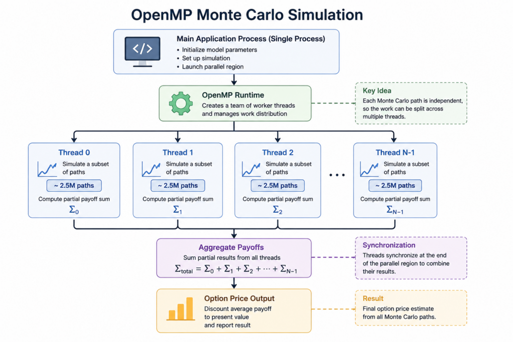
Monte Carlo pricing is a classic example of an embarrassingly parallel workload. By distributing simulation paths across multiple CPU cores, OpenMP can significantly reduce execution times with only a few additional lines of code.

Let’s create a “monte_carlo.cpp” file:

#include <omp.h>
#include <cmath>
#include <random>
#include <vector>
#include <iostream>

double simulate_option_price(
    double spot,
    double strike,
    double rate,
    double vol,
    double maturity,
    int num_paths)
{
    double payoff_sum = 0.0;

    #pragma omp parallel
    {
        std::mt19937 rng(42 + omp_get_thread_num());
        std::normal_distribution<> normal(0.0, 1.0);

        double local_sum = 0.0;

        #pragma omp for
        for (int i = 0; i < num_paths; ++i)
        {
            double z = normal(rng);

            double st =
                spot * std::exp(
                    (rate - 0.5 * vol * vol) * maturity +
                    vol * std::sqrt(maturity) * z);

            local_sum += std::max(st - strike, 0.0);
        }

        #pragma omp atomic
        payoff_sum += local_sum;
    }

    return std::exp(-rate * maturity) * payoff_sum / num_paths;
}

int main()
{
    double price = simulate_option_price(
        100.0,
        100.0,
        0.05,
        0.20,
        1.0,
        10'000'000);

    std::cout << "Option Price: " << price << '\n';
}

In the code above, each thread is responsible for a portion of the Monte Carlo simulations. Because individual simulation paths are completely independent, they can be executed concurrently on multiple CPU cores before their results are aggregated into a final option price estimate.

Compiling the Example

OpenMP is implemented through compiler support rather than as a standalone library. When the compiler encounters OpenMP directives such as #pragma omp parallel or #pragma omp for, it generates the necessary multithreaded code and links against the OpenMP runtime.

To compile the example using GCC:

g++ -O3 -fopenmp monte_carlo.cpp -o monte_carlo

The -fopenmp flag enables OpenMP support and links the OpenMP runtime library. Without this flag, the compiler will ignore the OpenMP directives and execute the code sequentially.

On macOS, the default Apple Clang compiler does not always include OpenMP support. In this case, developers typically install LLVM or GCC through Homebrew and compile the program using an OpenMP-enabled compiler.

Then execute the code:

./monte_carlo

The simulation above will be split on different threads before an aggregation step:

2.oneTBB

oneTBB (formerly Intel Threading Building Blocks) is a task-based parallel programming library created by Intel and first released in 2006. Rather than managing threads directly, developers express work as tasks, allowing oneTBB’s scheduler to efficiently distribute computation across multiple CPU cores.

Widely used in high-performance computing, quantitative finance, and scientific applications, oneTBB provides parallel algorithms, concurrent containers, and a work-stealing scheduler designed to simplify scalable multicore development.

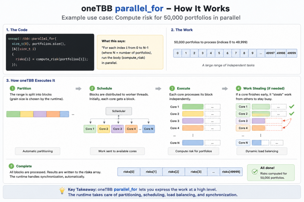
A bank needs to recompute a risk metric for 50,000 portfolios after a market move. Since each portfolio can be processed independently, the workload is naturally parallel. Instead of manually creating and managing threads, oneTBB distributes the portfolios across available CPU cores and balances the work automatically.

#include <oneapi/tbb/parallel_for.h>
#include <vector>

struct Portfolio
{
    std::string portfolio_id;
    std::vector<double> trade_dv01s;
};

double compute_risk(const Portfolio& portfolio)
{
    double dv01 = 0.0;

    for(double trade_dv01 : portfolio.trade_dv01s)
    {
        dv01 += trade_dv01;
    }

    return dv01;
}

int main()
{
    std::vector<Portfolio> portfolios(50000);
    std::vector<double> risks(portfolios.size());

    oneapi::tbb::parallel_for(
        size_t(0),
        portfolios.size(),
        [&](size_t i)
        {
            risks[i] = compute_risk(portfolios[i]);
        });

    return 0;
}

In this example, each portfolio can be evaluated independently, making the workload embarrassingly parallel. The parallel_for algorithm automatically divides the portfolio universe into smaller chunks and schedules them across available CPU cores. Unlike traditional thread-based approaches, developers do not need to manage thread creation, synchronization, or load balancing manually. This allows applications to scale efficiently on multicore systems while keeping the code concise and maintainable.

3.TaskFlow

Taskflow is a modern C++ parallel programming library that allows developers to express applications as task dependency graphs (DAGs) rather than individual threads or loops. It automatically schedules tasks, manages dependencies, and executes workflows efficiently across available CPU cores, making it particularly well-suited for data pipelines, simulations, and complex computational workflows. Taskflow is one the best C++ libraries for parallel programming.

The project was first presented publicly in 2019 as “Cpp-Taskflow: Fast Task-Based Parallel Programming Using Modern C++”.


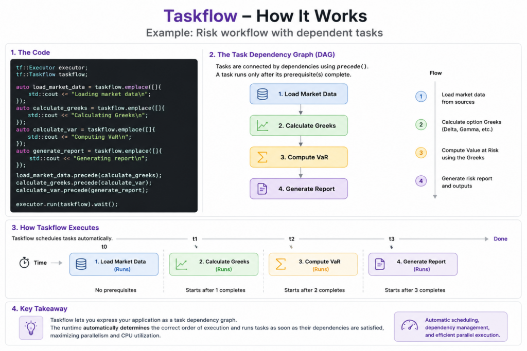
The following example models a simple risk analytics pipeline. Market data must be loaded before risk calculations can begin, while independent calculations can run in parallel. Once all computations are complete, a report is generated

#include <taskflow/taskflow.hpp>

int main() {

    tf::Executor executor;
    tf::Taskflow taskflow;

    auto load_market_data = taskflow.emplace([]{
        std::cout << "Loading market data\n";
    });

    auto calculate_greeks = taskflow.emplace([]{
        std::cout << "Calculating Greeks\n";
    });

    auto calculate_var = taskflow.emplace([]{
        std::cout << "Computing VaR\n";
    });

    auto generate_report = taskflow.emplace([]{
        std::cout << "Generating report\n";
    });

    load_market_data.precede(calculate_greeks);
    calculate_greeks.precede(calculate_var);
    calculate_var.precede(generate_report);

    executor.run(taskflow).wait();
}

Unlike OpenMP and oneTBB, which primarily focus on parallel loops and tasks, Taskflow allows developers to express entire applications as dependency graphs. Independent tasks can execute concurrently, while dependent tasks automatically wait for their prerequisites to complete. This approach is particularly useful for data pipelines, machine learning workflows, risk calculations, and other complex computational processes.

4.HPX

HPX is a modern C++ runtime system designed for scalable parallel and distributed applications. It extends the C++ standard library with asynchronous programming primitives such as futures, parallel algorithms, and task scheduling, allowing developers to write code that can scale from a laptop to a large computing cluster with minimal changes.

Typical Use Cases

  • Scientific computing
  • Distributed simulations
  • Numerical methods
  • Large-scale graph processing
  • HPC applications
  • Quantitative finance workloads requiring cluster-scale execution

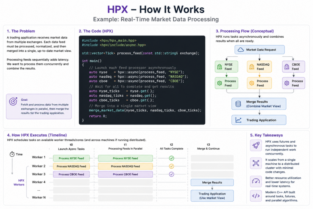
Imagine a trading platform receives market data from multiple exchanges. Instead of processing each feed sequentially, HPX can launch asynchronous tasks and combine the results once all feeds have been processed.

#include <hpx/hpx_main.hpp>
#include <hpx/include/async.hpp>

std::vector<Tick> process_feed(const std::string& exchange);

int main()
{
    auto nyse = hpx::async(process_feed, "NYSE");
    auto nasdaq = hpx::async(process_feed, "NASDAQ");
    auto cboe = hpx::async(process_feed, "CBOE");

    auto nyse_ticks = nyse.get();
    auto nasdaq_ticks = nasdaq.get();
    auto cboe_ticks = cboe.get();

    merge_market_data(
        nyse_ticks,
        nasdaq_ticks,
        cboe_ticks
    );
}

In this example, market data from multiple exchanges is processed concurrently using HPX futures. Each feed is handled asynchronously, allowing the application to utilize available computing resources efficiently while avoiding unnecessary blocking. Once all tasks complete, the results are merged into a unified market view.

In summary, HPX is one of the best C++ libraries for parallel programming!

5. A Summary of Pros and Cons

The libraries covered in this article address different parallel programming challenges, from simple loop parallelism to task scheduling, workflow orchestration, and distributed execution. The best choice depends on the complexity of your workload and how much control you need over execution.

LibraryStrengthsWeaknesses
OpenMPEasy to learn, simple loop parallelism, broad compiler supportLimited flexibility for complex task dependencies
oneTBBTask-based programming, automatic load balancing, scalable runtimeMore concepts to learn than OpenMP
TaskflowElegant workflow graphs (DAGs), intuitive dependency managementSmaller ecosystem and fewer learning resources
HPXFutures, asynchronous execution, distributed computing supportSteeper learning curve and more advanced programming model

Choosing the Right Library

  • OpenMP is ideal when you need to parallelize loops with minimal code changes.
  • oneTBB is a strong choice for applications composed of many independent tasks.
  • Taskflow excels at modelling complex workflows with explicit dependencies.
  • HPX is designed for highly scalable asynchronous applications that may span multiple machines.

In short: OpenMP focuses on loops, oneTBB on tasks, Taskflow on workflows, and HPX on asynchronous and distributed execution. Together, they represent a progression from straightforward multicore programming to advanced parallel and distributed systems.

June 11, 2026 0 comments
Llama.cpp Internals
AI

Llama.cpp Internals: The Secret Behind Fast LLMs

by cppforquants May 7, 2026

Modern AI is supposed to require massive GPUs, enormous cloud clusters, and billions of dollars in infrastructure. Yet somehow, llama.cpp can run surprisingly capable large language models on a laptop CPU, a MacBook, or even embedded hardware. In quant finance, low-latency systems are built around the same principles that make llama.cpp fast: cache efficiency, predictable memory access, SIMD acceleration, aggressive optimization, and minimizing unnecessary abstraction layers. High-frequency trading firms spend years optimizing nanoseconds out of market data pipelines, order routing systems, and pricing engines. Modern LLM inference is increasingly facing similar constraints. What are the secrets of the llama.cpp internals?

1.What is Lama.cpp?

llama.cpp is a high-performance C/C++ inference engine designed to run large language models (LLMs) efficiently on local hardware.

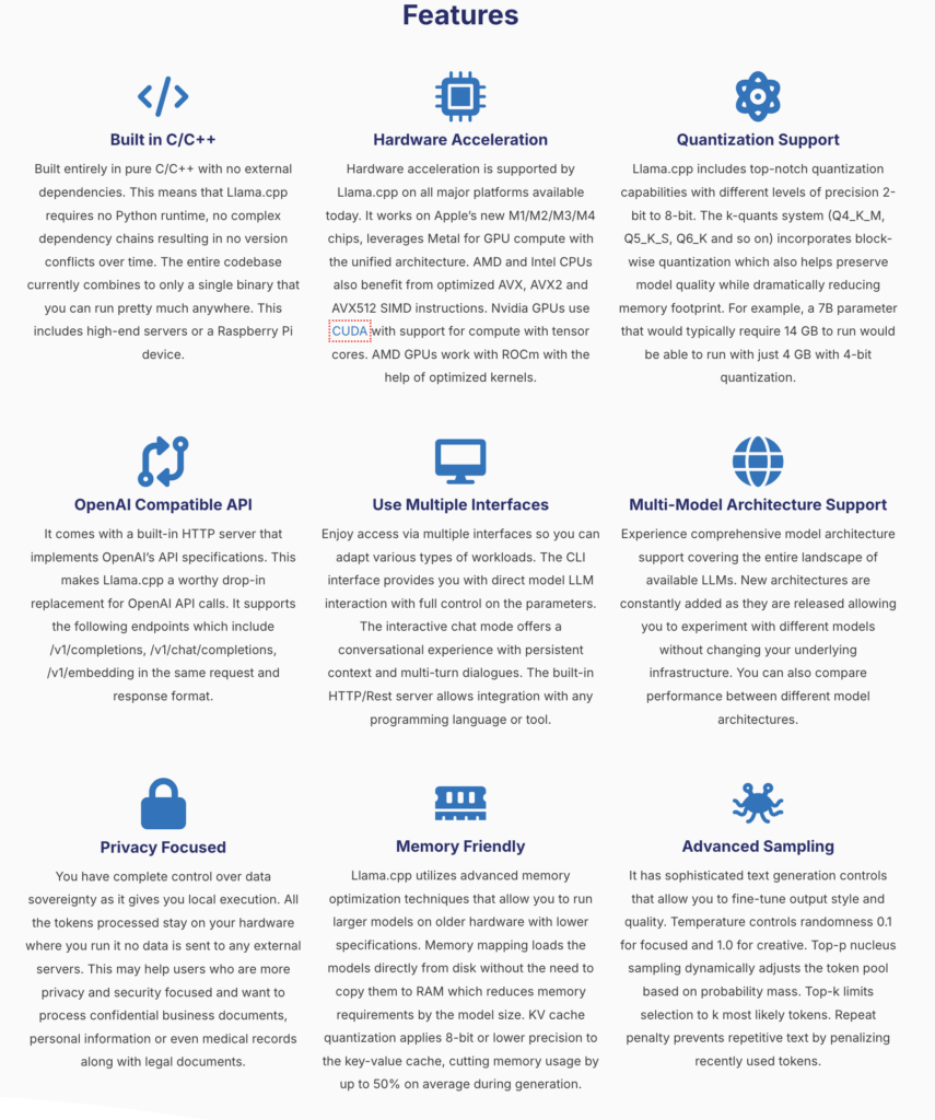
Originally created to run Meta’s LLaMA models on consumer CPUs, it has evolved into one of the most widely used runtimes for local AI inference. The features combine efficient quantization support, multi-model compatibility, advanced token sampling strategies, privacy-focused local inference, and highly optimized CPU/GPU execution.

2.What’s inside llama.cpp?

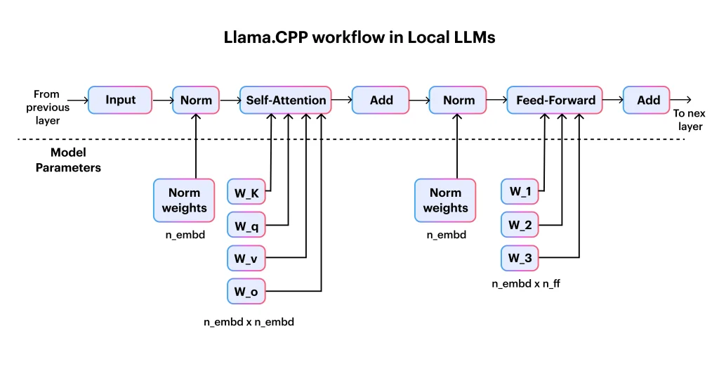
So, what are those llama.cpp internals? It begins with tokenization, where input text is split into discrete tokens and mapped to numerical IDs. These tokens are then converted into dense vector embeddings that represent semantic meaning in a form the model can efficiently process. The embeddings flow through the Transformer network, which is the core of the model and is responsible for most of the computation through stacked layers of self-attention and feed-forward operations. The Transformer outputs logits over the entire vocabulary, which are then passed through a sampling strategy to select the next token. This token is appended to the context, and the process repeats in an autoregressive loop until the output is complete.

To make this efficient on consumer hardware, llama.cpp relies on key systems-level optimizations such as quantized weights and the KV cache, which reuses previously computed attention states to avoid redundant work during long context generation.

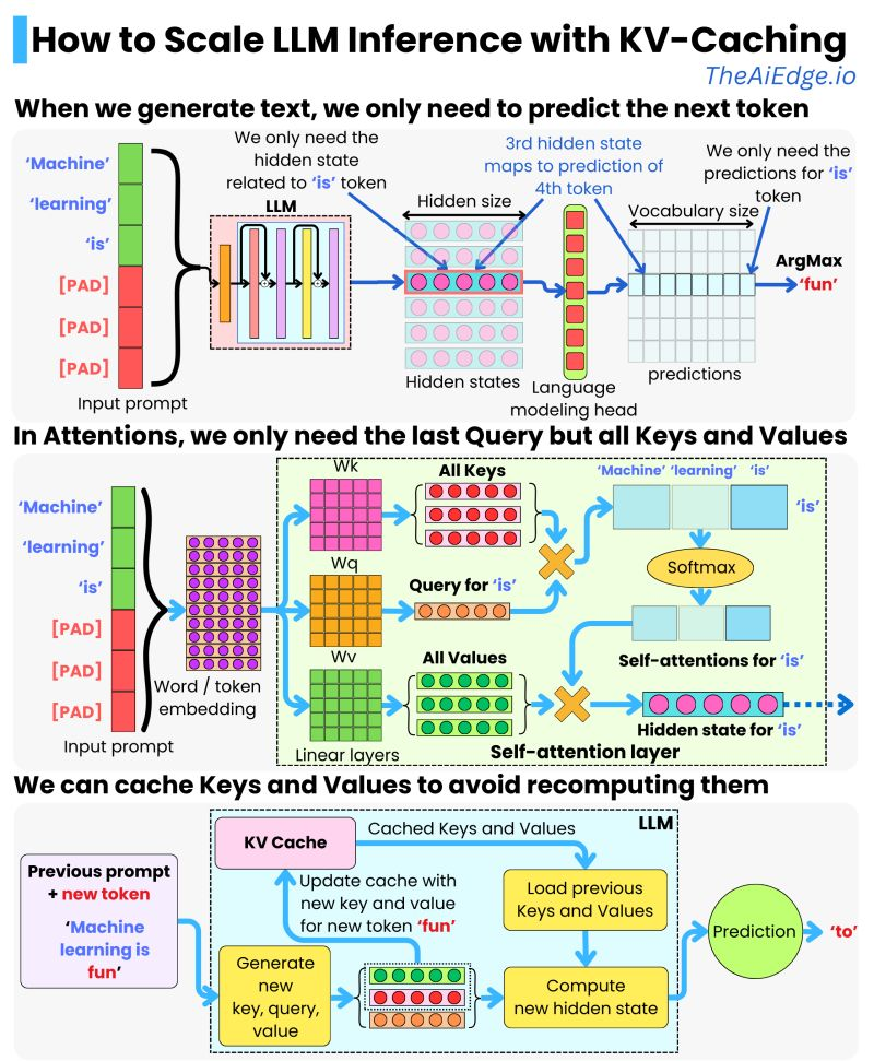
KV-Caching is really where the secret sauce is, avoiding to recompute the attention over the entire input sequence at every new token generation step by storing and reusing previously computed key and value tensors from earlier tokens:

The consequences on performance are impressive both in terms of latency:

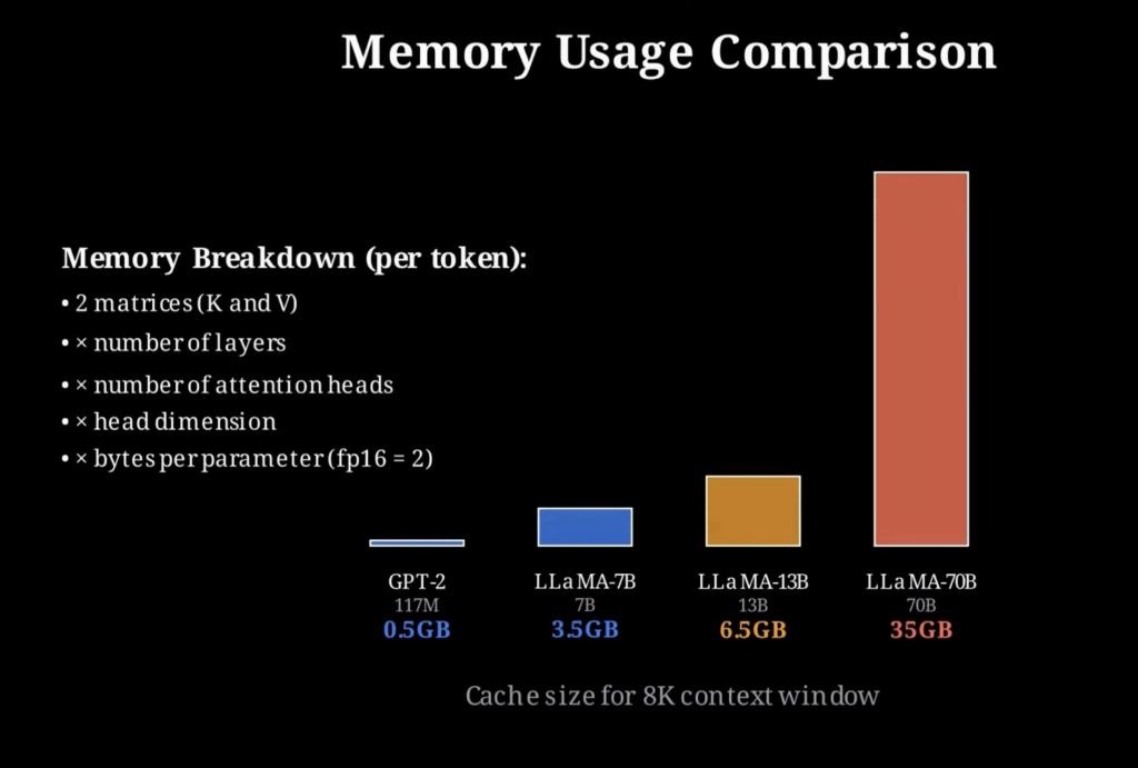
But there is no free lunch: the speed comes at the cost of increased memory usage, since the KV cache must store intermediate key and value tensors for every token in the context, and this footprint grows linearly with sequence length.

The breakdown of memory needed by token is unforgiving:

3.Install llama.cpp

You can install llama.cpp in a few different ways depending on whether you want control, speed of setup, or deployment flexibility.

The most common approach is to build it from source. This gives you full control over compilation flags and performance optimizations, and produces the core binaries like llama-cli and llama-server.

git clone https://github.com/ggml-org/llama.cpp
cd llama.cpp

cmake -B build
cmake --build build -j

Once built, you can immediately run a model using the CLI by pointing it to a GGUF file and providing a prompt for generation.

./build/bin/llama-cli -m models/model.gguf -p "Explain risk parity in finance" -n 200

If you want to skip compilation entirely, prebuilt binaries (when available for your platform) let you run inference directly. This is useful for quick testing or experimentation without setting up a build environment.

./llama-cli -m model.gguf -p "What is CAPM?" -n 200

For a more isolated and reproducible setup, you can run llama.cpp inside Docker. This avoids local dependency issues and is often used for deployment or server environments.

docker run -it --rm \
-v $(pwd)/models:/models \
ghcr.io/ggml-org/llama.cpp:latest \
llama-cli -m /models/model.gguf -p "Explain portfolio optimization" -n 200

To expose inference as a service, you can run the built-in server mode inside Docker and interact with it via HTTP, which is useful for integrating LLMs into applications or internal tools.

docker run -it --rm \
-p 8080:8080 \
-v $(pwd)/models:/models \
ghcr.io/ggml-org/llama.cpp:latest \
llama-server -m /models/model.gguf --host 0.0.0.0 --port 8080

You can then query it like a simple API endpoint, which is often how it is integrated into larger systems.

curl http://localhost:8080/completion -d '{
"prompt": "Explain Sharpe ratio",
"n_predict": 150
}'

On supported hardware, you can optionally enable GPU or accelerator backends during compilation to improve performance significantly. On Apple Silicon this uses Metal acceleration, while NVIDIA systems can use CUDA.

cmake -B build -DGGML_METAL=ON
cmake --build build -j

4. Some Use Cases for Quantitative Finance

In quantitative finance, llama.cpp internals matter and running models locally with llama.cpp is not about replacing trading systems, but about accelerating research, analysis, and decision support with low-latency, privacy-preserving inference.

One of the most immediate use cases is research assistance for strategy development. A local LLM can be used to explain or prototype ideas like portfolio optimization, factor models, or risk parity without sending sensitive research data to external APIs. Optimized llama.cpp internals play a big role!

Want to explain something in your portfolio optimization process?

./llama-cli -m model.gguf \
-p "Explain how mean-variance optimization is used in portfolio construction and derive the objective function" \
-n 300

Another practical use case is market microstructure analysis. Models can help summarize or interpret order book dynamics, liquidity conditions, or short-term price signals, which are often difficult to reason about quickly during research.

./llama-cli -m model.gguf \
-p "How does order book imbalance relate to short-term price movement in high-frequency trading?" \
-n 250

llama.cpp is also useful for risk analysis and scenario reasoning. Quant teams can use it to generate explanations or structured breakdowns of risk metrics, stress testing approaches, and portfolio exposure.

./llama-cli -m model.gguf \
-p "Compare VaR and CVaR and explain when each measure can fail under extreme market conditions" \
-n 300

A more advanced application is integrating llama.cpp into internal tools for research workflows. Since it can run as a local server, it can power internal copilots that sit next to proprietary datasets, allowing analysts to query models without exposing sensitive information externally.

./llama-server -m model.gguf --host 0.0.0.0 --port 8080

Finally, in low-latency environments, llama.cpp can be embedded directly into C++ systems for fast inference. While it is not used for execution-critical trading decisions, it can support real-time analytics, research dashboards, or decision-support tools where response time and data locality matter.

llama_model * model = llama_load_model_from_file("model.gguf", llama_model_default_params());
llama_context * ctx = llama_new_context_with_model(model, llama_context_default_params());

const char * prompt = "Explain pairs trading using a Kalman filter";
llama_eval(ctx, prompt, strlen(prompt), 0, 8);

char output[1024];
llama_get_next_token(ctx, output, sizeof(output));
printf("%s\n", output);

Overall, the value of llama.cpp in quantitative finance comes from its ability to bring LLM inference closer to the data and the system: reducing latency, improving privacy, and enabling tight integration with existing C++-based research and infrastructure stacks.

5. Alternatives to llama.cpp

While llama.cpp is one of the most popular runtimes for local LLM inference, especially on CPUs, there are several alternatives depending on whether you prioritize GPU throughput, production serving, or ecosystem tooling.

One major alternative is vLLM, which is designed for high-throughput GPU inference. It uses techniques like paged attention to efficiently manage memory during batching and is widely used in production LLM serving systems where throughput matters more than CPU efficiency.

pip install vllm

python -m vllm.entrypoints.openai.api_server \
--model meta-llama/Llama-3-8B-Instruct

Another option is TensorRT-LLM, which is highly optimized for NVIDIA GPUs. It focuses on maximizing inference speed using low-level kernel optimizations and is commonly used in enterprise-grade deployments where GPU performance is critical.

trtllm-build --model llama-3-8b
trtllm-run --engine model.engine

For more general-purpose deep learning workflows, PyTorch (with Hugging Face Transformers) remains the most flexible option. It is not optimized for CPU inference like llama.cpp, but it is widely used for prototyping, fine-tuning, and research.

from transformers import AutoModelForCausalLM, AutoTokenizer

model = AutoModelForCausalLM.from_pretrained("meta-llama/Llama-3-8B")
tokenizer = AutoTokenizer.from_pretrained("meta-llama/Llama-3-8B")

inputs = tokenizer("Explain portfolio optimization", return_tensors="pt")
outputs = model.generate(**inputs, max_new_tokens=200)

For Apple devices, MLX is an emerging alternative optimized specifically for Apple Silicon. It provides a more native experience on macOS compared to CUDA-centric stacks and is designed for efficient local inference.

import mlx_lm

model, tokenizer = mlx_lm.load("mlx-community/Llama-3-8B")
mlx_lm.generate(model, tokenizer, "Explain risk parity", max_tokens=200)

Finally, Ollama provides a higher-level abstraction over local LLMs, including llama.cpp under the hood in many cases. It focuses on developer experience, making it easy to run models locally with minimal setup.

ollama run llama3 "Explain the Sharpe ratio"

In summary:

  • llama.cpp → best for CPU inference, low-latency local systems, edge deployment thanks to llama.cpp internals
  • vLLM / TensorRT-LLM → best for high-throughput GPU serving
  • Transformers (PyTorch) → best for research and flexibility
  • MLX → best for Apple Silicon native performance
  • Ollama → best for simple developer experience

Each tool occupies a different layer of the LLM stack, from research flexibility to production-scale inference to lightweight local execution

May 7, 2026 0 comments
News

UK Banks Adopt Anthropic’s Mythos AI for Rapid Finance Insights

by cppforquants April 16, 2026

Headline-Style Summary: Anthropic’s Mythos AI Model to Debut for UK Banks Next Week, Signaling Potential Shift in Financial Landscape

As a quantitative analyst, I’ve been closely monitoring the emerging trends and signals in the finance data, and the recent announcement from Anthropic regarding the release of their Mythos AI model to UK financial institutions caught my attention. This development could potentially introduce new patterns and anomalies in the market, as the integration of advanced artificial intelligence capabilities into the financial sector may lead to shifts in trading strategies and investment decision-making.

Later in this article, we’ll delve into the details of Anthropic’s Mythos model and its potential impact, as well as explore other notable data-driven insights, such as the S&P 500 hitting an intraday all-time high and the AI trade’s potential to boost stocks while bonds remain cautious. By examining these quantitative signals, we can uncover valuable insights that may inform investment strategies and risk management in the evolving finance landscape.

🎥 Anthropic Says Mythos AI Model Available to UK Banks in ‘Next Week’ (Bloomberg)

As an investment strategist, the release of Anthropic’s Mythos AI model to UK financial institutions in the coming week presents both risks and opportunities. The model’s ability to spot cybersecurity vulnerabilities could be a valuable asset for banks, but the limited initial release suggests a cautious approach, potentially due to concerns about the model’s capabilities. The market sentiment appears to be one of cautious optimism, as the financial sector seeks to leverage the power of AI technology while managing the inherent risks. Investors will be closely watching the rollout of Mythos to see how it performs and how it is received by the UK banking industry.


🎥 Today on Taking Stock | S&P 500 Hits Intraday All-Time High (New York Stock Exchange)

As an investment strategist, I would frame this video as follows: The S&P 500’s recent surge to an intraday all-time high presents both opportunities and risks for investors. On the positive side, the market’s resilience in the face of ongoing economic uncertainty signals strong investor confidence and the potential for further upside. However, the lofty valuations and the possibility of increased volatility due to geopolitical tensions or policy shifts could pose challenges. Prudent investors should closely monitor market sentiment and be prepared to adjust their strategies accordingly. While the current market environment may offer attractive entry points, it is crucial to carefully weigh the risks and identify potential catalysts that could drive the next phase of the market’s performance.


🎥 Stocks Hit Record on Iran Ceasefire Hopes & TSMC Raises 2026 Outlook | Daybreak Europe 4/16/2026 (Bloomberg)

Global equities have reached record highs as investors regain confidence amid signs that Iran and the United States are considering a two-week extension to their ceasefire to allow more time for peace negotiations. This development, along with China’s robust economic growth and TSMC’s upbeat revenue forecast for 2026, have bolstered investor sentiment. The world’s top chipmaker, TSMC, has raised its revenue outlook for the year, underscoring the resilience of AI chip demand despite concerns over the economic impact of the Iran conflict. Institutional investors should closely monitor these key market drivers as they assess the investment landscape in the coming months.


🎥 AI Trade to Boost Stocks as Bonds Stay Cautious: 3-Minutes MLIV (Bloomberg)

The MLIV video provides a concise analysis of key market trends, highlighting the potential impact of AI trading on stock performance while cautioning about the cautious outlook for bonds. The report notes that global stocks have hit record levels on speculation of a ceasefire in Iran, while S&P futures indicate a positive start to the trading day. The Bank of England’s governor, Andrew Bailey, emphasizes that the central bank is in no rush to raise interest rates. The video’s focus on AI trading as a potential driver of stock gains underscores the importance of technological advancements in shaping investment strategies for decision-makers.


♟️ Interested in More?

  • Read the latest financial news: c++ for quants news.
April 16, 2026 0 comments
News

Oil Demand Decline and Iran Tensions: Navigating the Finance Landscape

by cppforquants April 14, 2026

Volatility in the global oil market has become a focal point of analysis, as recent geopolitical tensions in the Middle East have led to a surge in crude oil prices. The International Energy Agency’s latest report warns of a potential decline in global oil demand this year, as the price surge stemming from the regional conflict is expected to offset any growth. This dynamic will be a key factor to consider as we explore the video titled “IEA Warns of Global Oil Demand Decline Amid Iran War”.

Investor sentiment remains cautiously optimistic, with the prospect of a U.S.-Iran peace deal providing a glimmer of hope, as highlighted in the video “Today on Taking Stock | Investors Hold Out Hope for U.S.-Iran Peace Deal”. The potential for a resolution to the geopolitical tensions could have a significant impact on the trajectory of oil prices and global energy markets.

Turning our attention to the Asian markets, the video “Relief Rally in Asia Amid Renewed Hopes for Iran Peace Deal | Insight with Haslinda Amin 04/14/2026” suggests that the renewed hope for a peace deal has sparked a relief rally, underscoring the sensitivity of the region to developments in the Iran-U.S. conflict.

Furthermore, the video “US-Sanctioned Tanker Tests Trump’s Hormuz Blockade | Daybreak Europe 4/14/2026” highlights the ongoing tension in the Strait of Hormuz, a critical chokepoint for global oil transportation. The ability of sanctioned tankers to navigate this region could have significant implications for the supply and flow of crude oil, which will be crucial to monitor in the coming weeks and months.

🎥 IEA Warns of Global Oil Demand Decline Amid Iran War (Bloomberg)

The International Energy Agency warned that global oil demand will decline this year as a price surge caused by the Middle East conflict wipes out growth. The report highlights the market implications of the ongoing tensions in the region, which have led to a significant increase in oil prices and a corresponding decline in demand. The analysis provided by Bloomberg’s Anthony di Paola offers a concise and insightful assessment of the current situation, shedding light on the potential economic consequences of the geopolitical developments.


🎥 Today on Taking Stock | Investors Hold Out Hope for U.S.-Iran Peace Deal (New York Stock Exchange)

In the latest episode of “Taking Stock,” investors closely followed the ongoing negotiations between the United States and Iran, as the prospect of a potential peace deal continues to captivate global markets. The video delved into the complex geopolitical dynamics at play, exploring the potential economic implications of a successful resolution to the longstanding tensions between the two nations. Analysts highlighted the potential for a thawing of relations to unlock new investment opportunities, particularly in sectors that have been constrained by the existing sanctions regime. However, the presenters also cautioned that the path to a final agreement remains uncertain, underscoring the need for investors to closely monitor the evolving situation and its impact on broader market trends.


🎥 Relief Rally in Asia Amid Renewed Hopes for Iran Peace Deal | Insight with Haslinda Amin 04/14/2026 (Bloomberg)

The video segment highlights a relief rally in Asian markets amid renewed hopes for a peace deal with Iran. Viewers can observe a distinct pattern of investor calm and confidence, even as geopolitical tensions and market volatility persist. Insights from prominent industry leaders, such as the CEOs of M&G Asset Management and HSBC, offer quantitative signals on investor sentiment and risk management strategies during uncertain times. The analysis also delves into the broader economic implications, including the impact of the Russia-Ukraine war on energy security and investment trends in Malaysia.


🎥 US-Sanctioned Tanker Tests Trump’s Hormuz Blockade | Daybreak Europe 4/14/2026 (Bloomberg)

A US-sanctioned tanker linked to China is making its way through the Strait of Hormuz, testing President Donald Trump’s naval blockade. The tanker, Rich Starry, was blacklisted by Washington in 2023 for helping Tehran evade energy sanctions and is now making its second attempt in 24 hours to exit the Persian Gulf. This quantitative insight highlights an anomaly in the global energy market, as the US-sanctioned vessel challenges the Trump administration’s efforts to enforce its Hormuz blockade. The tanker’s movements and the potential impact on oil prices and geopolitical tensions will be closely watched by investors and policymakers alike.


♟️ Interested in More?

  • Read the latest financial news: c++ for quants news.
April 14, 2026 0 comments
News

Navigating Surging Markets: Insights from the U.S.-Iran Ceasefire

by cppforquants April 9, 2026

Quants will be closely watching the impact of the ceasefire between the U.S. and Iran, as the news has already sent markets surging. In a factual, investigative tone, this article will delve into the details of the truce and its implications for global financial markets. Later in the piece, we’ll present a range of relevant video content, including “Today on Taking Stock | Markets Surge on News of U.S.-Iran Ceasefire,” “Ceasefire Stirs Bets on Asian Currencies: 3-Minutes MLIV,” “Fragile US-Iran Truce; Israel Intensifies Lebanon Attacks | Horizons Middle East & Africa 4/9/2026,” and “Iran War: Vance to Lead Iran Talks as Tehran Says Ceasefire Violated | Daybreak Europe 4/9/2026,” to provide a comprehensive analysis of this developing story.

🎥 Today on Taking Stock | Markets Surge on News of U.S.-Iran Ceasefire (New York Stock Exchange)

The video provided a timely and insightful analysis of the recent surge in global financial markets, driven by the unexpected announcement of a ceasefire between the United States and Iran. The key financial themes highlighted included the significant impact of geopolitical tensions on market volatility, the role of investor sentiment in driving short-term price movements, and the importance of closely monitoring global political developments for their potential economic implications. The video’s expert commentary emphasized the need for investors to maintain a diversified portfolio and a long-term perspective, as sudden shifts in the geopolitical landscape can significantly influence the performance of various asset classes. Overall, the video offered a professional and informative perspective on the current state of the financial markets and the factors shaping their trajectory.


🎥 Ceasefire Stirs Bets on Asian Currencies: 3-Minutes MLIV (Bloomberg)

The video highlights the key financial themes surrounding the ceasefire in the region, and its potential significance for analysts and investors. The panel of experts from Bloomberg’s “The Opening Trade” discuss the implications of the ceasefire on Asian currencies, providing a concise and insightful analysis for the finance audience. The presentation offers a professional and clear overview of the video’s key takeaways, making it a valuable resource for those seeking to stay informed on the latest developments in the financial markets.


🎥 Fragile US-Iran Truce; Israel Intensifies Lebanon Attacks | Horizons Middle East & Africa 4/9/2026 (Bloomberg)

The video discusses the fragile ceasefire between the US and Iran, with Iran claiming that several terms of the agreement have been breached. The US is set to send a delegation led by Vice President JD Vance to Islamabad for talks on the matter. Additionally, the video highlights Israel’s intensified attacks on Hezbollah targets in Lebanon, as well as the rebound in oil prices after the biggest drop since 2020. The program features insights from experts, including a former senior US diplomat and investment professionals, on the regional dynamics and market implications.


🎥 Iran War: Vance to Lead Iran Talks as Tehran Says Ceasefire Violated | Daybreak Europe 4/9/2026 (Bloomberg)

As fighting continues in the Middle East, JD Vance will lead US-Iran talks in Islamabad this weekend, even as Tehran claims the ceasefire has been violated by Israeli strikes in Lebanon. Oil rebounded after its biggest one-day drop since April 2020, as the Strait of Hormuz remained largely blocked. Bloomberg has learned that the US wants specific commitments from its European allies on their pledge to help secure the Strait of Hormuz, following the US President’s criticism of NATO after his meeting with the alliance’s chief Mark Rutte in the White House.


♟️ Interested in More?

  • Read the latest financial news: c++ for quants news.
April 9, 2026 0 comments
News

Navigating Iran Tensions: Key Insights for Finance Professionals

by cppforquants April 7, 2026

The recent surge in geopolitical tensions between the United States and Iran has raised significant concerns among quantitative finance professionals. A technical analysis of market data reveals a notable increase in volatility across multiple asset classes, signaling heightened uncertainty and risk aversion among investors.

To provide deeper insights into this evolving situation, this article will feature a series of video segments. The first video, “Today on Taking Stock | U.S.-Iran Conflict Enters Sixth Week,” offers a comprehensive overview of the ongoing developments and their potential impact on global markets. Additionally, the “Trump’s Iran Ultimatum Heightens War Jitters | Insight with Haslinda Amin 04/07/2026” segment provides in-depth interviews and analysis from industry experts, shedding light on the complex geopolitical dynamics at play.

Furthermore, the “Risks Rise on Yet Another Iran Deadline: 3-Minutes MLIV” video presents a succinct, data-driven assessment of the potential risks and implications for quantitative traders and investors. Lastly, the “Trump’s Iran Deadline Looms; Tehran Rejects Proposal | Horizons Middle East & Africa 4/7/2026” segment explores the diplomatic efforts and potential outcomes of the escalating tensions between the United States and Iran.

By examining these video resources, readers will gain a comprehensive understanding of the current state of the U.S.-Iran conflict and its potential ramifications for the global financial markets.

🎥 Today on Taking Stock | U.S.-Iran Conflict Enters Sixth Week (New York Stock Exchange)

In the midst of ongoing global uncertainties, investors are closely monitoring the evolving situation between the United States and Iran, now entering its sixth week. As the geopolitical landscape continues to shift, market participants are assessing the potential implications for financial markets and the broader economy. While the path forward remains uncertain, prudent investors would be wise to stay informed and vigilant, as the ripple effects of this conflict could have far-reaching consequences. As we navigate these turbulent times, it will be crucial to maintain a disciplined, long-term approach and to closely follow the latest developments on this rapidly unfolding situation.


🎥 Trump’s Iran Ultimatum Heightens War Jitters | Insight with Haslinda Amin 04/07/2026 (Bloomberg)

The video provides an in-depth analysis of the heightened tensions between the United States and Iran, particularly surrounding President Trump’s ultimatum regarding navigation in the Strait of Hormuz. The program features interviews with prominent figures, including a Singapore minister and energy market experts, who discuss the potential implications of the situation for oil prices and global markets. The report also examines the broader geopolitical context, exploring the risk of military conflict and the potential for diplomatic resolution. Additionally, the video touches on the impact of the US-Iran tensions on other sectors, such as the performance of Samsung’s semiconductor business, which has seen strong growth despite the broader economic uncertainty.


🎥 Risks Rise on Yet Another Iran Deadline: 3-Minutes MLIV (Bloomberg)

The video’s content reflects the growing tensions surrounding the impending Iran deadline, with the potential for escalation in the ongoing geopolitical conflict. The discussion delves into the impact on Brent crude and oil prices, as well as the upcoming economic data releases, such as US PCE and CPI. These developments underscore the heightened risks and uncertainty facing analysts and investors in the current economic climate.


🎥 Trump’s Iran Deadline Looms; Tehran Rejects Proposal | Horizons Middle East & Africa 4/7/2026 (Bloomberg)

As an investment strategist assessing the video “Trump’s Iran Deadline Looms; Tehran Rejects Proposal | Horizons Middle East & Africa 4/7/2026,” the key risks, opportunities, and market sentiment can be highlighted as follows:

Risks: The escalating tensions between the US and Iran pose significant geopolitical risks, with the potential for military confrontation if Tehran continues to reject Trump’s demands. This could lead to disruptions in energy supply and price volatility in the Persian Gulf region, impacting global energy markets. Additionally, the involvement of other regional players, such as Israel’s strikes on Hezbollah infrastructure in Beirut, adds to the complexity and unpredictability of the situation.

Opportunities: The video features expert commentary from industry professionals, including Mehvish Ayub from Bank of Singapore, Karen Young from Columbia University’s Center on Global Energy Policy, and Neil Quilliam from Chatham House. Their insights on the regional dynamics and potential market implications could provide valuable information for investors seeking to navigate the uncertain landscape.

Market Sentiment: The market sentiment appears to be cautious, as investors closely monitor the developments between the US and Iran. The potential for further escalation and its impact on energy markets and regional stability are likely to be closely followed by investors. However, the return of the NASA Artemis astronauts from their record-breaking moon trip may offer a positive distraction and provide some optimism in the market.


♟️ Interested in More?

  • Read the latest financial news: c++ for quants news.
April 7, 2026 0 comments
Libraries

PMR Containers: Clean Memory Management in C++

by cppforquants April 3, 2026

Memory allocation is the silent tax on every high-frequency system. You profile your order book, strip out the obvious copies, tighten your cache lines — and still, somewhere in the flame graph, malloc is burning cycles you can’t afford. The problem isn’t always what you’re allocating; it’s how the allocator was chosen, usually once, at compile time, and buried so deep in your container types that changing it means rewriting half your data structures. In latency-sensitive code, that’s not a refactor — that’s a liability. What about PMR containers?

C++17’s std::pmr::polymorphic_allocator and the accompanying PMR container suite were designed precisely for this situation. The core idea is deceptively clean: decouple the container type from the memory resource it uses, and let that resource be swapped at runtime through a virtual dispatch layer thin enough to matter. A std::pmr::vector and a std::vector are structurally the same beast — but the PMR variant can draw from a monotonic arena, a synchronized pool, or your own custom resource, all without a template parameter change rippling through your entire call stack.

https://www.youtube.com/watch?v=SD9TcKPyfvc

For quant developers, this unlocks something genuinely practical. Your risk engine’s hot path can use a stack-backed arena during a pricing loop and fall back to the global heap everywhere else — same containers, same interfaces, zero allocation overhead where it counts.

What Is std::polymorphic_allocator and PMR containers?

Memory allocation in C++ has long been a source of friction: custom allocators existed since C++98, but their type-erased behavior was baked into the container’s template parameter, making std::vector<int, MyAlloc> and std::vector<int> entirely distinct, incompatible types. Passing them through a common interface required either templates everywhere or painful type erasure by hand.

C++17’s Polymorphic Memory Resource (PMR) library, under <memory_resource>, solves this by separating the allocation policy from the container type. The key abstraction is std::pmr::memory_resource, a pure virtual base class with two overridable primitives: do_allocate(size, alignment) and do_deallocate(ptr, size, alignment). Concrete resources — std::pmr::monotonic_buffer_resource, std::pmr::unsynchronized_pool_resource, and std::pmr::synchronized_pool_resource — implement these virtuals with different strategies.

std::pmr::polymorphic_allocator<T> wraps a memory_resource* and satisfies the standard Allocator requirements. Because all PMR containers are aliases like namespace pmr { using vector = std::vector<T, polymorphic_allocator<T>>; }, a std::pmr::vector<int> and another std::pmr::vector<int> using a different resource are the same type. You can store them in the same container, pass them to the same function, without templates.

std::array<std::byte, 4096> buf;
std::pmr::monotonic_buffer_resource pool{buf.data(), buf.size()};
std::pmr::vector<int> v{&pool};   // allocates from stack buffer

Chaining is possible: resources accept a fallback upstream resource, so monotonic_buffer_resource falls back to std::pmr::get_default_resource() (typically the heap) when the buffer exhausts.

Common pitfalls:

  • Lifetime hazard: the memory_resource* is a raw, non-owning pointer. If the resource is destroyed before the container, behavior is undefined.
  • Propagation semantics: polymorphic_allocator deliberately does not propagate on container copy (propagate_on_container_copy_assignment = false), so copies may silently use a different resource.
  • Nested containers: inner elements like std::pmr::string inside a std::pmr::vector only use the outer allocator if constructed with uses-allocator construction, which the standard library handles automatically — but custom types must opt in via std::uses_allocator.

PMR is ideal for arena-style allocation in hot paths, eliminating heap fragmentation with zero template proliferation.

Practical Use Case in Finance

Scenario: A high-frequency trading order book processes thousands of order updates per second. Each order carries metadata (tags, notes) stored in heap-allocated strings/vectors. Default allocators hit the global heap repeatedly, causing latency spikes. Using PMR with a stack-backed monotonic buffer eliminates most allocations during the hot path.

#include <memory_resource>
#include <vector>
#include <string>
#include <iostream>

// Order with PMR-aware string tags — no heap allocation during processing
struct Order {
    int id;
    double price;
    int quantity;
    // PMR string: allocator is injected, not baked into the type
    std::pmr::string symbol;
    std::pmr::vector<std::pmr::string> tags;

    Order(int id, double px, int qty, std::string_view sym,
          std::pmr::memory_resource* mr)
        : id(id), price(px), quantity(qty),
          symbol(sym, mr),          // uses the arena, not global heap
          tags(mr)                  // vector also uses the arena
    {}
};

int main() {
    // Stack buffer: 4 KB arena for one processing cycle
    alignas(std::max_align_t) std::byte buffer[4096];

    // Monotonic: bump-pointer allocator — O(1) alloc, zero per-object free
    std::pmr::monotonic_buffer_resource arena(buffer, sizeof(buffer));

    // PMR vector of Orders — all internal allocations flow through arena
    std::pmr::vector<Order> book(&arena);
    book.reserve(16);

    // Simulate ingesting orders in the hot loop
    for (int i = 0; i < 10; ++i) {
        Order& o = book.emplace_back(i, 100.0 + i * 0.25, 100, "AAPL", &arena);
        o.tags.emplace_back("aggressive", &arena);
        o.tags.emplace_back("marketable", &arena);
    }

    std::cout << "Processed " << book.size() << " orders from stack arena\n";
    // Arena destroyed here — single bulk release, no per-object free overhead
}

What this demonstrates: std::pmr::polymorphic_allocator decouples the allocation strategy from the container type. std::pmr::vector and std::pmr::string are the same types regardless of the backing resource — no template proliferation. The monotonic_buffer_resource turns hundreds of small allocations into a single stack bump, cutting allocator overhead to near-zero. At end-of-cycle, the arena resets in one shot, which is ideal for per-tick or per-batch processing patterns common in risk engines and market-data handlers.

Learn More: A Video Worth Watching

This CppCon 2017 talk by Alisdair Meredith provides essential context for understanding the design philosophy behind std::polymorphic_allocator and PMR containers. Meredith explores the evolution of C++’s allocator model and articulates the problems that polymorphic memory resources solve—particularly the need for runtime-configurable memory management without sacrificing performance. For quantitative finance developers, this perspective is invaluable: when managing massive datasets, optimizing memory allocation strategies directly impacts latency and throughput. The presentation clarifies how PMR containers enable sophisticated allocation patterns—such as pool allocators for microsecond-scale trading systems or custom allocators for NUMA-aware computing—all while maintaining type safety and avoiding virtual function overhead at the container level. Understanding the “why” behind these abstractions empowers you to architect more efficient data structures for demanding financial applications. Watch the full presentation to deepen your grasp of modern C++ memory management principles.

Conclusion

std::polymorphic_allocator and PMR containers represent a mature solution to a long-standing C++ problem: dynamic memory allocation without virtual function overhead or template bloat. By decoupling allocator policy from container type, PMR enables runtime flexibility while maintaining zero-cost abstraction—a rare combination.

The key takeaways are straightforward: use std::pmr::polymorphic_allocator when you need heterogeneous allocation strategies, leverage memory pools to reduce fragmentation, and embrace PMR containers in performance-critical codebases where every allocation matters.

For high-frequency trading systems and latency-sensitive financial platforms, PMR is transformative. You can now deploy a single compiled binary across environments with vastly different memory architectures—from NUMA systems to custom allocators backed by persistent memory—without recompilation. That flexibility, paired with predictable performance, is why PMR has become essential in production systems where milliseconds cost millions.

Start experimenting with std::pmr::monotonic_buffer_resource in your next project. The payoff compounds quickly.

Want to Go Deeper?

  • Explore more C++ feature articles: C++ for Quants — Features.
April 3, 2026 0 comments
  • 1
  • 2
  • 3
  • …
  • 11

@2025 - All Right Reserved.


Back To Top
  • Home
  • News
  • Contact
  • About