Bonds

In fixed income markets, the yield curve is a fundamental tool that maps interest rates to different maturities. It underpins the pricing of bonds, swaps, and other financial instruments. How to build a yield curve in C++?

Traders, quants, and risk managers rely on it daily to discount future cash flows. This article explores how to build a basic zero-coupon yield curve using C++, starting from market data and ending with interpolated discount factors. We’ll also compare our results with QuantLib, the industry-standard quantitative finance library.

1. What’s a Yield Curve?

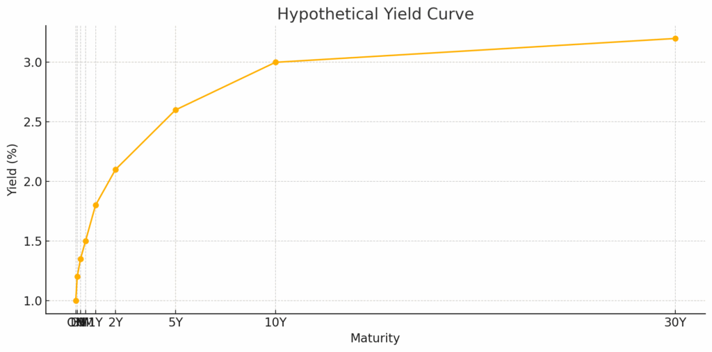
At its core, the yield curve captures how interest rates change with the length of time you lend money. Here’s an example of hypothetical yields across maturities:

Plotted on a graph, these points form the yield curve — typically upward sloping, as longer maturities usually command higher yields due to risk and time value of money.

However, in stressed environments, the curve can flatten or even invert (e.g., 2-year yield > 10-year yield), often signaling economic uncertainty:

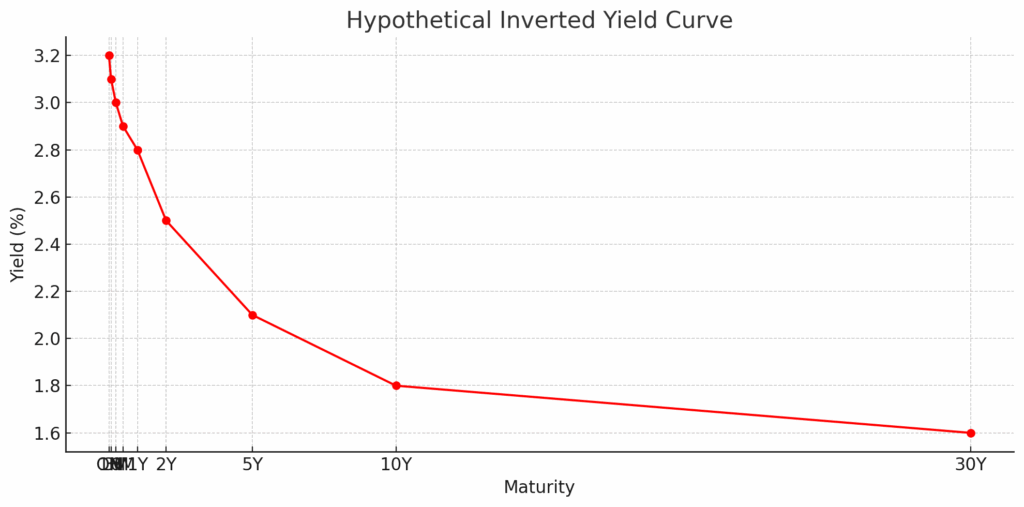
Here is the plot of a hypothetical inverted yield curve, where shorter-term yields are higher than longer-term ones. This often reflects market expectations of economic slowdown or interest rate cuts in the future.

When investors expect future economic weakness, they begin to anticipate interest rate cuts by the central bank. As a result:

• Demand increases for long-term bonds (seen as safe havens), which pushes their prices up and their yields down.
• Meanwhile, short-term rates may remain high due to current central bank policy (e.g. inflation control).

This flips the curve: short-term yields become higher than long-term yields.

2. Key Concepts Behind Yield Curve Construction

Before jumping into code, it’s important to understand how yield curves are built from market data. In practice, we don’t observe a complete yield curve directly, we build (or “bootstrap”) it from liquid instruments such as:

• Deposits (e.g., overnight to 6 months)
• Forward Rate Agreements (FRAs) and Futures
• Swaps (e.g., 1-year to 30-year)

These instruments give us information about specific points on the curve. QuantLib uses these to construct a continuous curve using interpolation (e.g., linear, log-linear) between observed data points.

Some essential building blocks in QuantLib include:

• RateHelpers: Abstractions that turn market quotes (like deposit or swap rates) into bootstrapping constraints.
• DayCount conventions and Calendars: Needed for accurate date and interest calculations.
• YieldTermStructure: The central object representing the term structure of interest rates, which you can query for zero rates, discount factors, or forward rates.

QuantLib lets you define all of this in a modular way, so you can plug in market data and generate an accurate, arbitrage-free curve for pricing and risk analysis.

3. Implement in C++ with Quantlib

To construct a yield curve in QuantLib, you’ll typically bootstrap it from a mix of deposit rates and swaps. QuantLib provides a flexible interface to handle real-world instruments and interpolate the curve. Below is a minimal C++ example that constructs a USD zero curve from deposit and swap rates:

#include <ql/quantlib.hpp>
#include <iostream>

using namespace QuantLib;

int main() {
    Calendar calendar = UnitedStates(UnitedStates::GovernmentBond);
    Date today(25, June, 2025);
    Settings::instance().evaluationDate() = today;

    // Market quotes
    Rate depositRate = 0.015; // 1.5% for 3M deposit
    Rate swapRate5Y = 0.025;  // 2.5% for 5Y swap

    // Quote handles
    Handle<Quote> dRate(boost::make_shared<SimpleQuote>(depositRate));
    Handle<Quote> sRate(boost::make_shared<SimpleQuote>(swapRate5Y));

    // Day counters and conventions
    DayCounter depositDayCount = Actual360();
    DayCounter curveDayCount = Actual365Fixed();
    Thirty360 swapDayCount(Thirty360::BondBasis);

    // Instrument helpers
    std::vector<boost::shared_ptr<RateHelper>> instruments;

    instruments.push_back(boost::make_shared<DepositRateHelper>(
        dRate, 3 * Months, 2, calendar, ModifiedFollowing, false, depositDayCount));

    instruments.push_back(boost::make_shared<SwapRateHelper>(
        sRate, 5 * Years, calendar, Annual, Unadjusted, swapDayCount,
        boost::make_shared<Euribor6M>()));

    // Construct the yield curve
    boost::shared_ptr<YieldTermStructure> yieldCurve =
        boost::make_shared<PiecewiseYieldCurve<ZeroYield, Linear>>(
            today, instruments, curveDayCount);

    // Example output: discount factor at 2Y
    Date maturity = calendar.advance(today, 2, Years);
    std::cout << "==== Yield Curve ====" << std::endl;
    for (int y = 1; y <= 5; ++y) {
    Date maturity = calendar.advance(today, y, Years);
    double discount = yieldCurve->discount(maturity);
    double zeroRate = yieldCurve->zeroRate(maturity, curveDayCount, Compounded, Annual).rate();

    std::cout << "Maturity: " << y << "Y\t"
              << "Yield: " << std::fixed << std::setprecision(2) << 100 * zeroRate << "%\t"
              << "Discount: " << std::setprecision(5) << discount
              << std::endl;
    }

    return 0;
}

This snippet shows how to:

• Set up today’s date and calendar,
• Define deposit and swap instruments as bootstrapping inputs,
• Build a PiecewiseYieldCurve using QuantLib’s helper classes,
• Query the curve for a discount factor.

You can easily extend this with more instruments (FRA, futures, longer swaps) for a realistic curve.

4. Compile, Execute and Plot

After installing quantlib, I compile my code with the following CMakeLists.txt:

cmake_minimum_required(VERSION 3.10)
project(QuantLibImpliedVolExample)

set(CMAKE_CXX_STANDARD 17)

find_package(PkgConfig REQUIRED)
pkg_check_modules(QUANTLIB REQUIRED QuantLib)

include_directories(${QUANTLIB_INCLUDE_DIRS})
link_directories(${QUANTLIB_LIBRARY_DIRS})

add_executable(yieldcurve ../yieldcurve.cpp)
target_link_libraries(yieldcurve ${QUANTLIB_LIBRARIES})

I run:

mkdir build
cd build
cmake ..
make

And run:

➜ build ./yieldcurve
==== Yield Curve ====
Maturity: 1Y Yield: 1.68% Discount: 0.98345
Maturity: 2Y Yield: 1.89% Discount: 0.96324
Maturity: 3Y Yield: 2.10% Discount: 0.93946
Maturity: 4Y Yield: 2.31% Discount: 0.91272
Maturity: 5Y Yield: 2.52% Discount: 0.88306

And we can plot it too:

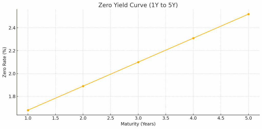
So this is the plot of the zero yield curve from 1 to 5 years, based on your QuantLib output. It shows a smooth, gently upward-sloping curve: typical for a healthy interest rate environment.

But why is it so… Linear?

This is due to both the limited number of inputs and the interpolation method applied.

In the example above, the curve is built using QuantLib’s PiecewiseYieldCurve<ZeroYield, Linear>, which performs linear interpolation between the zero rates of the provided instruments. With only a short-term and a long-term point, this leads to a straight-line interpolation between the two, hence the linear shape.

In reality, yield curves typically exhibit curvature:

• They rise steeply in the short term,
• Then gradually flatten as maturity increases.

This reflects the market’s expectations about interest rates, inflation, and economic growth over time.

To better approximate real-world behavior, the curve can be constructed using:

• A richer set of instruments (e.g., deposits, futures, swaps across many maturities),
• More appropriate interpolation techniques such as LogLinear or Cubic.

5. A More Realistic Curve

This version uses LogLinear interpolation, which interpolates on the log of the discount factors. It results in a more natural term structure than simple linear interpolation, even with only two instruments.

For a truly realistic curve, additional instruments should be incorporated, especially swaps with intermediate maturities:

#include <ql/quantlib.hpp>
#include <iostream>
#include <iomanip>

using namespace QuantLib;

int main() {
    Calendar calendar = UnitedStates(UnitedStates::GovernmentBond);
    Date today(25, June, 2025);
    Settings::instance().evaluationDate() = today;

    // Market quotes
    Rate depositRate = 0.015;    // 1.5% for 3M deposit
    Rate swapRate2Y = 0.020;     // 2.0% for 2Y swap
    Rate swapRate5Y = 0.025;     // 2.5% for 5Y swap
    Rate swapRate10Y = 0.030;    // 3.0% for 10Y swap

    // Quote handles
    Handle<Quote> dRate(boost::make_shared<SimpleQuote>(depositRate));
    Handle<Quote> sRate2Y(boost::make_shared<SimpleQuote>(swapRate2Y));
    Handle<Quote> sRate5Y(boost::make_shared<SimpleQuote>(swapRate5Y));
    Handle<Quote> sRate10Y(boost::make_shared<SimpleQuote>(swapRate10Y));

    // Day counters and conventions
    DayCounter depositDayCount = Actual360();
    DayCounter curveDayCount = Actual365Fixed();
    Thirty360 swapDayCount(Thirty360::BondBasis);

    // Instrument helpers
    std::vector<boost::shared_ptr<RateHelper>> instruments;

    instruments.push_back(boost::make_shared<DepositRateHelper>(
        dRate, 3 * Months, 2, calendar, ModifiedFollowing, false, depositDayCount));

    instruments.push_back(boost::make_shared<SwapRateHelper>(
        sRate2Y, 2 * Years, calendar, Annual, Unadjusted, swapDayCount,
        boost::make_shared<Euribor6M>()));

    instruments.push_back(boost::make_shared<SwapRateHelper>(
        sRate5Y, 5 * Years, calendar, Annual, Unadjusted, swapDayCount,
        boost::make_shared<Euribor6M>()));

    instruments.push_back(boost::make_shared<SwapRateHelper>(
        sRate10Y, 10 * Years, calendar, Annual, Unadjusted, swapDayCount,
        boost::make_shared<Euribor6M>()));

    // Construct the yield curve with Cubic interpolation
    boost::shared_ptr<YieldTermStructure> yieldCurve =
        boost::make_shared<PiecewiseYieldCurve<ZeroYield, Cubic>>(
            today, instruments, curveDayCount);

    // Output: yield curve at each year from 1Y to 10Y
    std::cout << "==== Yield Curve ====" << std::endl;
    for (int y = 1; y <= 10; ++y) {
        Date maturity = calendar.advance(today, y, Years);
        double discount = yieldCurve->discount(maturity);
        double zeroRate = yieldCurve->zeroRate(maturity, curveDayCount, Compounded, Annual).rate();

        std::cout << "Maturity: " << y << "Y\t"
                  << "Yield: " << std::fixed << std::setprecision(2) << 100 * zeroRate << "%\t"
                  << "Discount: " << std::setprecision(5) << discount
                  << std::endl;
    }

    return 0;
}

And let’s run it again:

➜  build ./yieldcurve
==== Yield Curve ====
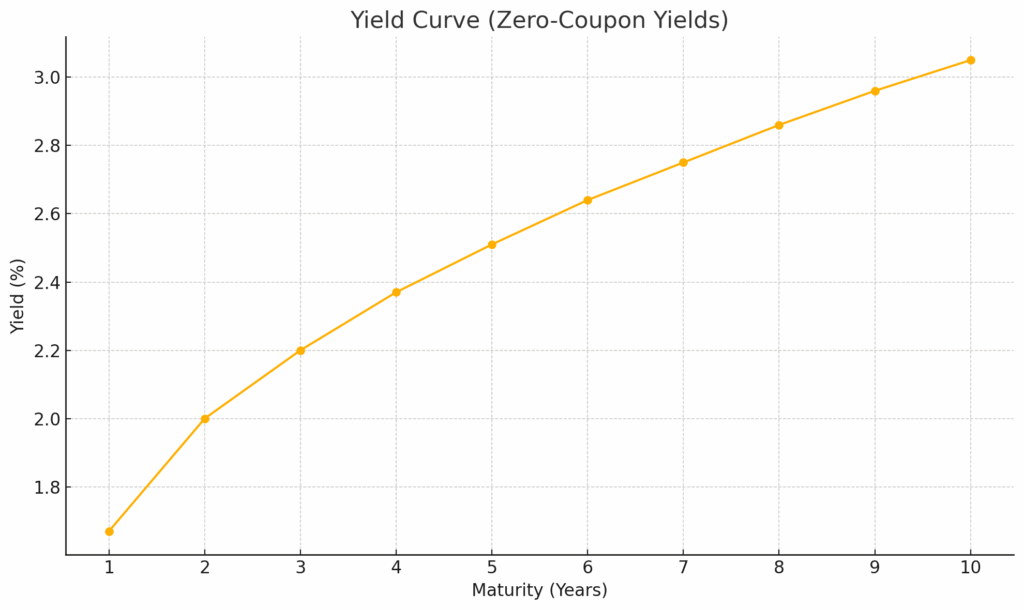
Maturity: 1Y    Yield: 1.67%    Discount: 0.98355
Maturity: 2Y    Yield: 2.00%    Discount: 0.96122
Maturity: 3Y    Yield: 2.20%    Discount: 0.93680
Maturity: 4Y    Yield: 2.37%    Discount: 0.91058
Maturity: 5Y    Yield: 2.51%    Discount: 0.88320
Maturity: 6Y    Yield: 2.64%    Discount: 0.85524
Maturity: 7Y    Yield: 2.75%    Discount: 0.82674
Maturity: 8Y    Yield: 2.86%    Discount: 0.79790
Maturity: 9Y    Yield: 2.96%    Discount: 0.76912
Maturity: 10Y   Yield: 3.05%    Discount: 0.74018

Which gives a better looking yield curve:

Bond pricing is a fundamental skill for any quant. Whether you’re managing fixed-income portfolios or calculating risk metrics, understanding how a bond is priced is essential. In this article, we’ll walk through the core formula, explore how clean and dirty prices differ, and implement it in C++ using QuantLib. How to build a bonds pricer?

1.The Bond Pricing Formula

When you buy a bond, you’re essentially buying a stream of future cash flows: fixed coupon payments and the return of the face value at maturity. The price you pay for that stream depends on how much those future payments are worth today — in other words, their present value.

🔹 The Dirty Price: What You’re Really Paying

The dirty price (or full price) is the total value of the discounted future cash flows:

[math] \Large{\text{Dirty Price} = \sum_{i=1}^{N} \frac{C_i}{(1 + y)^{t_i}}} [/math]

Where:

• [math]C_i[/math] is the cash flow at time [math]t_i[/math] — typically the coupon, and the last cash flow includes the face value.
• [math]y[/math] is the periodic yield, i.e., the annual yield divided by the number of coupon payments per year.
• [math]t_i[/math] is the year fraction between today and the [math]i^\text{th}[/math] payment, calculated using day count conventions (like Actual/360, 30/360, etc.).

In simpler terms: money in the future is worth less than money today, and the discounting reflects that.

🔹 Accrued Interest: What You Owe the Seller

Most bonds trade between coupon dates, meaning the seller has already “earned” part of the next coupon. To make things fair, the buyer compensates them via accrued interest:

[math] \Large \text{Accrued Interest} = \text{Coupon} \times \frac{\text{Days since last payment}}{\text{Days in period}} [/math]

So if you buy the bond halfway through the coupon cycle, you’ll owe the seller half the coupon. This ensures the next payment (which you’ll receive in full) is properly split based on ownership time.

🔹 Clean Price: The Market Quote

Bond prices are typically quoted clean, without accrued interest:

[math] \Large \text{Clean Price} = \text{Dirty Price} – \text{Accrued Interest} [/math]

This keeps things tidy when quoting and trading, and lets the system calculate accrued interest automatically behind the scenes.

Together, these three equations form the backbone of bond pricing. In the next section, we’ll show how QuantLib brings them to life — no need to write your own discounting engine.

3. Setting Up the Bond in QuantLib

Now that we’ve covered the theory behind bond pricing, let’s see how to implement it using QuantLib. One of QuantLib’s biggest strengths is how it mirrors the real-world structure of financial instruments — every component reflects a real aspect of how bonds are modeled, priced, and managed in production systems.

Here’s what we need to set up a bond in QuantLib:

📅 Calendar, Date, and Schedule

• Calendar: Tells QuantLib which days are business days. This is crucial for calculating coupon dates and settlement dates correctly. We’ll use TARGET(), a commonly used calendar for euro-denominated instruments.
• Date: QuantLib’s custom date class used to define evaluation, issue, maturity, and coupon dates.
• Schedule: Automatically generates all coupon dates between the start and maturity dates. You specify the frequency (e.g., semiannual), the calendar, and how to adjust dates if they fall on weekends or holidays.

In other words: this trio defines when things happen.

💵 FixedRateBond

• This is the actual bond object.
• It takes in:
  • Settlement days (e.g., T+2),
  • Face value (e.g., 1000),
  • The coupon schedule,
  • The fixed coupon rate(s),
  • Day count convention (e.g., Actual/360),
  • Date adjustment rules.
• Once constructed, it contains all the future cash flows, knows when they occur, and how much they are.

Think of FixedRateBond as your contractual definition of the bond.

📈 YieldTermStructure

• This represents the discount curve.
• You can define it using:
  • A flat yield (e.g., 4.5% across all maturities),
  • A bootstrap from market instruments (swaps, deposits, etc.),
  • Or even a custom curve from CSV or historical data.
• QuantLib uses this curve to discount each cash flow to present value.

This is your interest rate environment — essential for pricing.

🧠 DiscountingBondEngine

• This is the pricing engine: the part of QuantLib that ties it all together.
• Once you set the bond’s pricing engine to a DiscountingBondEngine, it knows how to price it using the curve.
• It computes:
  • The dirty price,
  • The clean price,
  • The accrued interest,
  • And other risk measures like duration and convexity.

You can think of it as the calculator that applies all the math we just discussed.

4. Implementation

Let’s implement:

#include <ql/quantlib.hpp>
#include <iostream>
#include <iomanip>

using namespace QuantLib;

int main() {
    // Set the evaluation date
    Date today(24, June, 2025);
    Settings::instance().evaluationDate() = today;

    // Bond parameters
    Real faceValue = 1000.0;
    Rate couponRate = 0.05; // 5%
    Date maturity(24, June, 2030);
    Frequency frequency = Semiannual;
    Integer settlementDays = 2;
    DayCounter dayCounter = Actual360();
    BusinessDayConvention convention = Unadjusted;
    Calendar calendar = TARGET();

    // Build the schedule of coupon payments
    Schedule schedule(today, maturity, Period(frequency), calendar,
                      convention, convention, DateGeneration::Backward, false);

    // Create the fixed-rate bond
    FixedRateBond bond(settlementDays, faceValue, schedule,
                       std::vector<Rate>{couponRate}, dayCounter, convention);

    // Build a flat yield curve (4.5%)
    Handle<YieldTermStructure> yieldCurve(
        boost::make_shared<FlatForward>(today, 0.045, dayCounter));

    // Set the pricing engine using the discounting curve
    bond.setPricingEngine(boost::make_shared<DiscountingBondEngine>(yieldCurve));

    // Output the results
    std::cout << std::fixed << std::setprecision(2);
    std::cout << "Clean Price   : " << bond.cleanPrice() << std::endl;
    std::cout << "Dirty Price   : " << bond.dirtyPrice() << std::endl;
    std::cout << "Accrued Interest: " << bond.accruedAmount() << std::endl;

    return 0;
}

After compilation and run, we get:

➜  build ./pricer  
Clean Price   : 102.01
Dirty Price   : 102.04
Accrued Interest: 0.03

🔹 Clean Price = 102.01

This is the market-quoted price of the bond, excluding any interest that has accrued since the last coupon date.
It means that the bond is trading at 102.01% of its face value — i.e., £1,020.10 for a bond with a £1,000 face value.

🔹 Dirty Price = 102.04

This is the actual amount you’d pay if you bought the bond today.
It includes both:

• The clean price (102.01), and
• The interest the seller has “earned” since the last coupon.

So:

[math]
\text{Dirty Price} = \text{Clean Price} + \text{Accrued Interest} = 102.01 + 0.03 = 102.04
[/math]

🔹 Accrued Interest = 0.03

This is the amount of coupon interest that has accrued since the last coupon date but hasn’t been paid yet.
The buyer pays this to the seller because the seller has held the bond for part of the current coupon period.

In your case, it’s 0.03% of face value, or £0.30 on a £1,000 bond — meaning you’re very close to the previous coupon date.