Data Structures

You’ve probably heard traders talk about the order book before: it’s one of the most fundamental tools in modern markets. It’s a very important tool for traders, analysts or quants. A trading order book is a real-time record of all buy and sell orders for a financial asset, like a stock, bond, or cryptocurrency, organized by price level. How does it work and why does it matter?

What’s a Trading Order Book?

An order book is a real-time, organized list of buy and sell orders for a financial asset, arranged by price level and volume. It reflects market depth: the amount of demand and supply available at each price.

In essence:

• Buy orders (bids): traders wanting to purchase, listed from highest to lowest price.
• Sell orders (asks): traders wanting to sell, listed from lowest to highest price.

Each entry includes a price and a quantity. When a buy and sell order meet at the same price, a trade executes, removing both from the book.

The best bid is the highest price someone will pay.
The best ask is the lowest price someone will sell for.
The spread is the difference between the two — a key measure of liquidity.

Order books help traders understand supply, demand, and short-term price movements, forming the foundation for price discovery in modern markets.

How Does it Work?

This image illustrates how an order book works by showing the interaction between buyers (bids) and sellers (asks) for a currency pair.

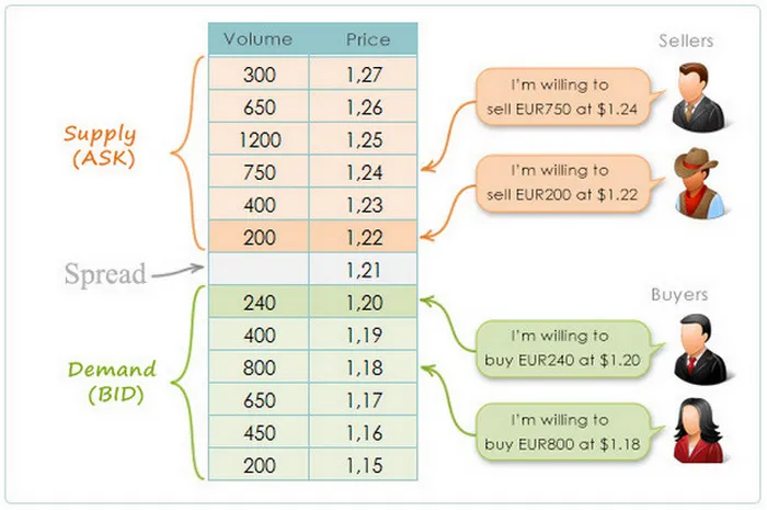
On the right, you see two groups of participants:

• Sellers (Supply / ASK) list the prices at which they’re willing to sell.
• Buyers (Demand / BID) list the prices at which they’re willing to buy.

The table in the middle displays these orders:

• The top half (orange) represents sell orders. Each row shows a price and the volume available at that price. For example, one seller wants to sell EUR 200 at $1.22, another EUR 750 at $1.24.
• The bottom half (green) represents buy orders. For instance, a buyer wants to buy EUR 240 at $1.20, another EUR 800 at $1.18.

Between them lies the spread, the small gap between the highest bid (best buyer) and the lowest ask (best seller). In this example, the spread is $0.01 (between $1.20 and $1.21).

This spread reflects the liquidity and balance of supply and demand — tighter spreads usually mean a more liquid market. When a market order arrives, it executes at the best available price from these existing limit orders, causing the market price to update.

The Importance of the Bid-Ask Spread

The spread is the gap between the best ask (lowest price a seller accepts) and the best bid (highest price a buyer offers).
It represents the cost of immediacy: how much extra a trader pays to buy right now or how much less they get to sell immediately.

A tight spread means a liquid, competitive market with many buyers and sellers.
A wide spread suggests uncertainty, low liquidity, or higher risk.

For pricers, the spread is both a signal and a target.
They aim to quote prices that are competitive enough to attract trades but wide enough to cover risks.
Too narrow, and they might lose money to fast market moves.
Too wide, and they risk losing flow to other participants.

So, pricers constantly adjust their spreads based on volatility, order flow, inventory, and competition balancing profitability with market presence.

How To Implement a Trading Order Book in C++?

Here’s a compact blueprint for a limit-order book in C++: data layout, core ops, and gotchas. We will:

• Maintain two sides: bids (max-first) and asks (min-first).
• Group orders by price level; within a level, keep FIFO (price–time priority).
• Keep a fast index from order_id → node/iterator to support O(1) cancel/replace.
• Use integer ticks (e.g., cents, pips) — avoid floating point for prices.

using OrderId   = uint64_t;
using Qty       = int64_t;        // signed for partial fills math
using Px       = int64_t;         // price in ticks
enum Side { Buy, Sell };

struct Order {
  OrderId id;
  Side side;
  Px price;
  Qty qty;            // remaining
  uint64_t ts;        // exchange/seq time for tie-breaks
  // intrusive list pointers for O(1) erase
  Order* prev = nullptr;
  Order* next = nullptr;
};

struct Level {
  Px price;
  Order* head = nullptr;
  Order* tail = nullptr;
  inline void push_back(Order* o);
  inline void erase(Order* o);
  bool empty() const { return head == nullptr; }
};

// price → level; bids need descending, asks ascending
using BookSide = std::map<Px, Level, std::greater<Px>>;     // bids
using BookSideAsk = std::map<Px, Level, std::less<Px>>;     // asks

struct OrderBook {
  BookSide bids;
  BookSideAsk asks;
  std::unordered_map<OrderId, Order*> by_id;  // direct handle for cancel/replace

  // API
  void add_limit(OrderId id, Side side, Px px, Qty qty, uint64_t ts);
  void cancel(OrderId id);
  void replace(OrderId id, Px new_px, Qty new_qty, uint64_t ts); // cancel+add semantics
  void match_market(Side side, Qty qty);
  // helpers
  Level& level(BookSide& s, Px px);
  Level& level(BookSideAsk& s, Px px);
};

The C++ order book example keeps two ordered maps: one for bids (descending prices) and one for asks (ascending). Each price level stores a queue of orders to preserve price–time priority. Each order holds its ID, side, price (as an integer tick), quantity, and pointers to neighboring orders for quick removal. A

n additional hash map links every order ID to its memory address, allowing O(1) cancellation or modification. When a new limit order arrives, it matches existing orders on the opposite side if the prices overlap; otherwise, it’s added to the appropriate queue. Market orders consume orders starting from the best available price. The design avoids floating-point precision issues by using integers, and it minimizes heap allocations through object pooling. Operations within a price level run in constant time, while finding the best price is logarithmic. The result is a fast, deterministic system that mirrors how real exchanges match and update orders.

The Challenges for Pricers: Find the Mid

For pricers, one of the core challenges is finding the true mid-price: the fair point between supply and demand. In theory, the mid is simply the average of the best bid and best ask, but in practice it’s far more complex. The visible quotes in the order book might not reflect real interest, as large traders often hide size or layer orders strategically.

The mid can also move rapidly in volatile markets, making it difficult for pricers to keep up without overreacting to noise. Liquidity imbalances, or instance, when one side of the book is much deeper than the other, distort the apparent equilibrium. Moreover, different trading venues might show slightly different best prices, forcing pricers to aggregate data across markets.

Latency adds another layer of uncertainty: by the time data is received, the true mid might have shifted. Pricers must therefore estimate a “synthetic mid”, balancing recent trades, book depth, and volatility signals. Their goal is to quote competitively around this mid without exposing themselves to adverse selection. The challenge lies in constantly adapting: finding the mid not as a static number, but as a moving, data-driven target that defines the heartbeat of market making.

How to Develop a Pricer: Train an ML Model to Predict the Mid

Developing a pricer that uses machine learning to estimate the mid-price involves combining market microstructure knowledge with careful model design. The goal is to predict the true or future mid (the fair value where supply and demand balance) based on high-frequency order book data.

The process starts with data collection: capturing snapshots of the limit order book, trades, and quote updates with precise timestamps. Each snapshot provides features such as best bid/ask, spread, market depth, imbalance (volume difference between bid and ask sides), last trade direction, and short-term volatility. These become the inputs to the model.

Next comes labeling. A common choice is the future mid, for example the mid-price 1–5 seconds ahead. This trains the model to learn short-term price dynamics rather than just the current quote.

The model selection depends on latency and interpretability requirements. For low-latency environments, ML models like gradient-boosted trees (like XGBoost or LightGBM) work well. For richer patterns, temporal architectures such as CNNs, LSTMs, or Transformers on order book sequences capture evolving microstructure dynamics.

Once trained, the model’s predicted mid becomes the reference for quoting: bids are set slightly below and asks slightly above it, adjusted for volatility, inventory, and risk tolerance.

The main challenges lie in data quality, microsecond synchronization, feature drift, and ensuring the model generalizes under changing market regimes. Continuous retraining and real-time monitoring are essential. In essence, the ML pricer learns to “feel” the market’s equilibrium — a constantly shifting target driven by flow, depth, and momentum.

Conclusion

In conclusion, an order book is the foundation of market mechanics, recording all buy and sell intentions that together form price discovery. The spread, the gap between the best bid and ask, reflects market liquidity and trading costs — a narrow spread means efficiency, while a wide one signals risk or low activity. For pricers, managing and interpreting that spread is crucial: they must stay competitive while protecting against adverse moves. Finding the true mid between supply and demand is not trivial; it fluctuates constantly with market depth, hidden orders, and volatility. Modern pricers therefore rely on machine learning models to estimate the fair or future mid, using features like order-book imbalance, volume, and trade flow. These models learn to sense microstructure dynamics and help automate quoting decisions in real time. Building such systems is both a technical and strategic challenge, requiring clean data, synchronized feeds, fast inference, and constant retraining to stay aligned with a living, breathing market.

Since C++11, smart pointers have become essential tools for managing memory safely and efficiently.
They eliminate the need for manual new/delete while enabling shared or exclusive ownership semantics. What are smart pointers for C++ financial data?

1. Raw Pointers vs Smart Pointers: The Evolution

C++ traditionally relied on raw pointers (T*) for dynamic memory management. While flexible, raw pointers come with risks: memory leaks, dangling references, and double deletes — especially in complex quant systems where ownership isn’t always clear.

Smart pointers, introduced in C++11, offer a safer alternative by wrapping raw pointers with automatic lifetime management.

C++11 introduced smart pointers, which wrap raw pointers with automatic memory management based on ownership models:

• std::unique_ptr<T>: sole ownership, cannot be copied.
• std::shared_ptr<T>: shared ownership via reference counting.
• std::weak_ptr<T>: non-owning reference to break cycles.
• std::make_shared<T>() / std::make_unique<T>(): factory functions for safe allocation.

Consider this classic raw pointer pattern, here with a dummy YieldCurve object:

YieldCurve* curve = new YieldCurve(...);
// use curve
delete curve; // ❌ must remember to call this, or risk a leak

With std::shared_ptr, you simplify and secure ownership:

auto curve = std::make_shared<YieldCurve>(...); // ✅ deleted automatically when last owner goes out of scope

2. Heap-Allocated Financial Structures and Smart Pointers

In financial systems, data structures like price histories, risk vectors, or trade buckets are often heap-allocated.

It’s either because of their size or because they need to be shared across multiple components or threads. Managing their lifetime correctly is crucial to avoid memory leaks or invalid access.

Let’s take a practical example of such structures: std::vector. A vector is stored on the stack, while its internal elements are managed on the heap.

void computePnL() {
    std::vector<double> pnl = {120.5, -75.2, 30.0};  // stack-allocated vector
    double total = 0.0;
    for (double p : pnl) {
        total += p;
    }
    std::cout << "Total PnL: " << total << std::endl;
} // ✅ `pnl` is automatically destroyed when it goes out of scope

So a value-based vector would look like this in memory:

The stack contains basic metadata about the vector and a pointer to the heap block where the values are actually defined.

How would a vector smart shared pointer look like?

It would be a pointer defined on the stack pointing to a vector object on the heap that contains a pointer towards the actual values also on the heap. Yes, it’s a bit nested!

When the last std::shared_ptr to a heap-allocated object goes out of scope or is reset, the internal reference count drops to zero.

At that moment, unlike raw pointers, the managed object (in this case, the std::vector<double>) is automatically destroyed, and its memory is released. This ensures safe, deterministic cleanup without manual delete calls.

Let’s see with an example for shared pointers:

#include <iostream>
#include <memory>
#include <vector>

void createVector() {
    auto pnl = std::make_shared<std::vector<double>>(std::initializer_list<double>{120.5, -75.2, 30.0});
    std::cout << "Inside createVector(), use_count: " << pnl.use_count() << std::endl;
} // 🔥 When pnl goes out of scope, vector is destroyed (ref count drops to 0)

int main() {
    createVector();
    std::cout << "Back in main()" << std::endl;
}

When pnl goes out of scope, vector is destroyed (ref count drops to 0) automatically.

Now, let’s talk about std::unique_ptr<T>:

While shared_ptr supports shared ownership with reference counting, unique_ptr enforces strict single ownership.

It cannot be copied, only moved making ownership transfer explicit and safe.

#include <iostream>
#include <memory>
#include <vector>

std::unique_ptr<std::vector<double>> createVector() {
    auto pnl = std::make_unique<std::vector<double>>(std::initializer_list<double>{100.0, -20.0, 50.0});
    std::cout << "Inside createVector(), vector size: " << pnl->size() << std::endl;
    return pnl; // ownership is transferred (moved) to the caller
}

int main() {
    auto vecPtr = createVector(); // vecPtr now owns the vector
    std::cout << "Back in main(), first value: " << vecPtr->at(0) << std::endl;

    // auto copy = vecPtr; ❌ This won't compile: unique_ptr cannot be copied
    auto moved = std::move(vecPtr); // ✅ Ownership moved
    if (!vecPtr)
        std::cout << "vecPtr is now null after move.\n";
}

This shows how unique_ptr ensures exclusive ownership: once moved, the original pointer becomes null, and the resource is safely destroyed when the final owner goes out of scope.

Now, let’s talk about std::weak_ptr<T>:

Unlike shared_ptr, a weak_ptr does not contribute to the reference count. It’s designed for non-owning references that safely observe a shared_ptr, managed resource, especially useful to break cyclic references in shared ownership scenarios (like parent ↔ child graphs or caches).

Here’s a minimal example:

#include <iostream>
#include <memory>
#include <vector>

void observeVector() {
    std::shared_ptr<std::vector<int>> data = std::make_shared<std::vector<int>>(std::initializer_list<int>{1, 2, 3});
    std::weak_ptr<std::vector<int>> weakData = data; // 👀 weak observer

    std::cout << "use_count: " << data.use_count() << std::endl;

    if (auto locked = weakData.lock()) { // Try to temporarily access
        std::cout << "Accessed value: " << locked->at(0) << std::endl;
    }
    
    data.reset(); // destroy the shared_ptr

    if (auto locked = weakData.lock()) {
        std::cout << "Still alive.\n";
    } else {
        std::cout << "Resource expired.\n";
    }
}

std::weak_ptr is ideal for temporary, non-owning access to a shared resource. It lets you safely check if the object is still alive without extending its lifetime: perfect for avoiding cyclic references and building efficient observers or caches.

Said differently: std::weak_ptr is a smart pointer specifically designed to observe the lifecycle of a std::shared_ptr without affecting its ownership or reference count.

3. Overhead of Using Smart Pointers in HFT

While smart pointers offer safety and convenience, they do introduce runtime overhead, especially std::shared_ptr.

🏎️ unique_ptr, by contrast, is zero-overhead in release builds — it’s just a thin RAII wrapper around a raw pointer with no reference counting.

🔁 shared_ptr maintains a reference count (typically via an internal control block). Each copy or reset updates this count atomically, which adds thread-safe synchronization costs.

🔒 weak_ptr shares this control block, adding some memory overhead, though access via .lock() is generally efficient.

In performance-critical, low-latency systems (e.g. HFT), overuse of shared_ptr can introduce cache pressure and latency spikes. It’s crucial to profile and use them only where ownership semantics justify the cost.

Each std::shared_ptr has an associated control block (on the heap) storing:

• use_count (shared references)
• weak_count

Every copy, assignment, or destruction updates use_count atomically:

std::shared_ptr<T> a = b;  // atomic increment

These atomic ops:

• May invalidate CPU cache lines
• Cause false sharing if multiple threads access nearby memory
• Require synchronization fences, introducing latency

Each shared_ptr object requires a heap allocation for its control block. This:

• Adds malloc/free overhead
• Increases memory fragmentation
• May cause non-contiguous accesses, leading to cache misses

Also, destroying a shared_ptr with many references (e.g., in a tree or graph) may lead to:

• Long chain deletions
• Blocking deallocation spikes
• Potential STW-like moments under multi-threaded pressure

4. Summary

Here’s a clear summary table of the key points we’ve covered:

The code for the article is available here:

https://github.com/cppforquants/smartpointers/tree/main

Sequential containers in C++ store elements in a linear order, where each element is positioned relative to the one before or after it. They’re designed for efficient iteration, fast access, and are typically used when element order matters, such as in time-based data.

The most commonly used sequential containers in the STL are:

• std::vector: dynamic array with contiguous memory
• std::deque: double-ended queue with fast insertions/removals at both ends
• std::array: fixed-size array on the stack
• std::list / std::forward_list: linked lists

In quantitative finance, sequential containers are often at the heart of systems that process tick data, historical time series, price paths, and rolling windows. When processing millions of data points per day, the choice of container directly impacts latency, memory usage, and cache performance.

1. std::vector: The Workhorse

std::vector is a dynamic array container in C++. It’s one of the most performance-critical tools in a quant developer’s toolbox — especially for time-series data, simulation paths, and numerical computations.

🧠 Stack vs Heap: The Memory Model

In C++, memory is managed in two primary regions:

🔸 A std::vector behaves as follows:

• The vector object itself (pointer, size, capacity) lives on the stack.
• The elements it stores live in a dynamically allocated heap buffer.

💡 Consequences:

• You can create a std::vector of size 1 million without stack overflow.
• But heap allocation is slower than stack and can cause fragmentation if misused.
• When passed by value, only the stack-held metadata is copied (until you access elements).

📦 Contiguous Memory Layout

A std::vector stores all its elements in a single, contiguous block of memory on the heap — just like a C-style array.

Why this matters:

• CPU cache efficiency: Memory is prefetched in blocks — sequential access is blazing fast.
• Enables pointer arithmetic, SIMD (Single Instruction Multiple Data), and direct interfacing with C APIs.

💥 For quants: When you’re processing millions of floats/doubles (e.g., price histories, simulation paths), contiguous memory layout can be a 10× performance multiplier vs pointer-chasing containers like std::list.

⏱ Time Complexity

⚠️ When capacity is exhausted, std::vector reallocates, usually doubling its capacity and copying all elements — which invalidates pointers and iterators.

💻 Example: Using std::vector for Rolling Average on Price Time Series

#include <vector>
#include <numeric>  // for std::accumulate

int main() {
    // Simulated price time series (e.g. 1 price per second)
    std::vector<double> prices;

    // Simulate appending tick data
    for (int i = 0; i < 10'000'000; ++i) {
        prices.push_back(100.0 + 0.01 * (i % 100)); // Fake tick data
    }

    // Compute rolling average over the last 5 prices
    size_t window_size = 5;
    std::vector<double> rolling_avg;

    for (size_t i = window_size; i < prices.size(); ++i) {
        double sum = std::accumulate(prices.begin() + i - window_size, prices.begin() + i, 0.0);
        rolling_avg.push_back(sum / window_size);
    }

    // Print the last rolling average
    std::cout << "Last rolling avg: " << rolling_avg.back() << std::endl;

    return 0;
}

🧠 Key Points:

• std::vector<double> stores prices in contiguous heap memory, enabling fast iteration.
• push_back appends elements efficiently until capacity needs to grow.
• Access via prices[i] or iterators is cache-friendly.
• This method is fast but not optimal for rolling computations — a future section will show how std::deque or a circular buffer improves performance here.

2. std::deque: Double-Ended Queue

std::deque stands for “double-ended queue” — a general-purpose container that supports efficient insertion and deletion at both ends. Unlike std::vector, which shines in random access, std::deque is optimized for dynamic FIFO (first-in, first-out) or sliding window patterns.

🧠 Stack vs Heap: Where Does Data Live?

• Like std::vector, the std::deque object (its metadata) lives on the stack.
• The underlying elements are allocated on the heap — but not contiguously.

💡 Consequences:

• You can append or prepend large amounts of data without stack overflow.
• Compared to std::vector, memory access is less cache-efficient due to fragmentation.

📦 Contiguous Memory? No.

Unlike std::vector, which stores all elements in one continuous memory block, std::deque allocates multiple fixed-size blocks (typically 4KB–8KB) and maintains a map (array of pointers) to those blocks.

Why this matters:

• Appending to front/back is fast, since it just adds blocks.
• But access patterns may be less cache-friendly, especially in tight loops.

⏱ Time Complexity

⚠️ Internally more complex: uses a segmented memory model (think: mini-arrays linked together via pointer table).

⚙️ What’s Under the Hood?

A simplified mental model:

cppCopierModifierT** block_map;   // array of pointers to blocks
T* blocks[N];    // actual blocks on the heap

• Each block holds a fixed number of elements.
• deque manages which block and offset your index points to.

✅ Strengths

• Fast insertion/removal at both ends (O(1)).
• No expensive shifting like vector.
• Stable references to elements even after growth at ends (unlike vector).

⚠️ Trade-offs

• Not contiguous → worse cache locality than vector.
• Random access is constant time, but slightly slower than vector[i].
• Slightly higher memory overhead due to internal structure (block map + block padding).

📈 Quant Finance Use Cases

• Rolling windows on tick or quote streams (e.g. sliding 1-minute buffer).
• Time-based buffers for short-term volatility, VWAP, or moving averages.
• Event-driven systems where data is both consumed and appended continuously.

Example:

std::deque<double> price_buffer;
// push_front for new tick, pop_back to discard old

💬 Typical Interview Questions

1. “How would you implement a rolling average over a tick stream?”
   • A good answer involves std::deque for its O(1) append/remove at both ends.
2. “Why not use std::vector if you’re appending at the front?”
   • Tests understanding of std::vector‘s O(n) front-insertion cost vs deque‘s O(1).
3. “Explain the memory layout of deque vs vector, and how it affects performance.”
   • Looks for awareness of cache implications.

💻 Code Example: Rolling Average with std::deque

cppCopierModifier#include <iostream>
#include <deque>
#include <numeric>

int main() {
    std::deque<double> price_window;
    size_t window_size = 5;

    for (int i = 0; i < 10; ++i) {
        double new_price = 100.0 + i;
        price_window.push_back(new_price);

        // Keep deque size fixed
        if (price_window.size() > window_size) {
            price_window.pop_front();  // Efficient O(1)
        }

        if (price_window.size() == window_size) {
            double avg = std::accumulate(price_window.begin(), price_window.end(), 0.0) / window_size;
            std::cout << "Rolling average: " << avg << std::endl;
        }
    }

    return 0;
}

🧠 Summary: deque vs vector

3. std::array: Fixed-Size Array

std::array is a stack-allocated, fixed-size container introduced in C++11. It wraps a C-style array with a safer, STL-compatible interface while retaining zero overhead. In quant finance, it’s ideal when you know the size at compile time and want maximum performance and predictability.

🧠 Stack vs Heap: Where Does Data Live?

• std::array stores all of its data on the stack — no dynamic memory allocation.
• The container itself is the data, unlike std::vector or std::deque, which hold pointers to heap-allocated buffers.

💡 Consequences:

• Blazing fast allocation/deallocation — no malloc, no heap overhead.
• Extremely cache-friendly — everything is packed in a single memory block.
• But: limited size (you can’t store millions of elements safely).

📦 Contiguous Memory? Yes.

std::array maintains a true contiguous layout, just like a C array. This enables:

• Fast random access via arr[i]
• Compatibility with C APIs
• SIMD/vectorization-friendly memory layout

⏱ Time Complexity

⚙️ What’s Under the Hood?

Conceptually:

cppCopierModifiertemplate<typename T, std::size_t N>
struct array {
    T elems[N];  // Inline data — lives on the stack
};

• No dynamic allocation.
• No capacity concept — just a fixed-size C array with better syntax and STL methods.

✅ Strengths

• Zero runtime overhead — allocation is just moving the stack pointer.
• Extremely fast access and iteration.
• Safer than raw arrays — bounds-safe with .at() and STL integration (.begin(), .end(), etc.).

⚠️ Trade-offs

• Fixed size — can’t grow or shrink at runtime.
• Risk of stack overflow if size is too large.
• Pass-by-value is expensive (copies all elements) unless using references.

📈 Quant Finance Use Cases

• Grids for finite difference/PDE solvers: std::array<double, N>
• Precomputed factors (e.g., Greeks at fixed deltas)
• Fixed-size historical feature vectors for ML signals
• Small matrices or stat buffers in embedded systems or hot loops

// Greeks for delta hedging
std::array<double, 5> greeks = { 0.45, 0.01, -0.02, 0.005, 0.0001 };

💬 Typical Interview Questions

1. “What’s the difference between std::array, std::vector, and C-style arrays?”
   • Tests understanding of memory layout, allocation, and safety.
2. “When would you prefer std::array over std::vector?”
   • Looking for “when size is known at compile time and performance matters.”
3. “What’s the risk of using large std::arrays?”
   • Looking for awareness of stack overflow and memory constraints.

💻 Code Example: Option Grid for PDE Solver

int main() {
    constexpr std::size_t N = 5; // e.g. 5 grid points in a discretized asset space
    std::array<double, N> option_values = {100.0, 101.5, 102.8, 104.2, 105.0};

    // Simple finite-difference operation: delta = (V[i+1] - V[i]) / dx
    double dx = 1.0;
    for (std::size_t i = 0; i < N - 1; ++i) {
        double delta = (option_values[i + 1] - option_values[i]) / dx;
        std::cout << "delta[" << i << "] = " << delta << std::endl;
    }

    return 0;
}

🧠 Summary: std::array vs vector/deque

4. std::list / std::forward_list: Linked Lists

std::list and std::forward_list are the C++ STL’s doubly- and singly-linked list implementations. While rarely used in performance-critical quant finance applications, they are still part of the container toolkit and may shine in niche situations involving frequent insertions/removals in the middle of large datasets — but not for numeric data or tight loops.

🧠 Stack vs Heap: Where Does Data Live?

• Both containers are heap-based: each element is dynamically allocated as a separate node.
• The container object itself (head pointer, size metadata) is on the stack.
• But the actual elements — and their pointers — are spread across the heap.

💡 Consequences:

• Extremely poor cache locality.
• Each insertion allocates heap memory → slow.
• Ideal for predictable insertion/removal patterns, not for numerical processing.

📦 Contiguous Memory? Definitely Not.

Each element is a node containing:

• The value
• One (std::forward_list) or two (std::list) pointers

So memory looks like this:

[Node1] → [Node2] → [Node3] ...   (or doubly linked)

💣 You lose any benefit of prefetching or SIMD. Iteration causes pointer chasing, leading to cache misses and latency spikes.

⏱ Time Complexity

⚙️ What’s Under the Hood?

Each node contains:

• value
• next pointer (and prev for std::list)

So conceptually:

Node {
    T value;
    Node* next; // and prev, if doubly linked
};

• std::list uses two pointers per node.
• std::forward_list is lighter — just one pointer — but can’t iterate backward.

✅ Strengths

• Efficient insertions/removals anywhere — no element shifting like vector.
• Iterator-stable: elements don’t move in memory.
• Predictable performance for queue-like workloads with frequent mid-stream changes.

⚠️ Trade-offs

• Terrible cache locality — each node is scattered.
• No random access — everything is via iteration.
• Heavy memory overhead: ~2×–3× the size of your data.
• Heap allocation per node = slow.

📈 Quant Finance Use Cases (Rare/Niche)

• Managing a priority-sorted list of limit orders (insert/delete in mid-stream).
• Event systems where exact insertion position matters.
• Custom allocators or object pools in performance-tuned engines.

Usually, in real systems, this is replaced by:

• std::deque for queues
• std::vector for indexed data
• Custom intrusive lists if performance really matters

💬 Typical Interview Questions

1. “What’s the trade-off between std::vector and std::list?”
   • Looking for cache locality vs insert/delete performance.
2. “How would you store a stream of operations that require arbitrary insert/delete?”
   • Tests knowledge of when to use linked lists despite their cost.
3. “Why is std::list usually a bad idea for numeric workloads?”
   • Looking for insight into heap fragmentation and CPU cache behavior.

💻 Code Example: Linked List of Events

#include <iostream>
#include <list>

struct TradeEvent {
    double price;
    double quantity;
};

int main() {
    std::list<TradeEvent> event_log;

    // Simulate inserting trades
    event_log.push_back({100.0, 500});
    event_log.push_back({101.2, 200});
    event_log.push_front({99.5, 300});  // Insert at front

    // Iterate through events
    for (const auto& e : event_log) {
        std::cout << "Price: " << e.price << ", Qty: " << e.quantity << std::endl;
    }

    return 0;
}

🧠 Summary: std::list / std::forward_list

Unless you need fast structural changes mid-stream, these containers are rarely used in quant systems. But it’s important to know when and why they exist.