Greeks

In quantitative finance, understanding how an option’s value changes over time is critical for risk management and trading. This is where Theta, the Greek that measures time decay, plays a central role. In this article, you’ll learn how to calculate Theta for options in C++ with a simple yet powerful approach to estimate how much an option’s price erodes as it approaches expiration. Whether you’re building a pricing engine or just deepening your understanding of the Greeks, this guide will walk you through a practical C++ implementation step-by-step.

1. What is Theta?

Theta is one of the most important Greeks in options trading. It measures the rate at which an option loses value as time passes, assuming all other factors remain constant. This phenomenon is known as time decay.

Mathematically, Theta is defined as the partial derivative of the option price V with respect to time t:

[math]\large \Theta = \frac{\partial V}{\partial t}[/math]

In most practical cases, Theta is negative for long option positions meaning the value of the option decreases as time progresses. This reflects the diminishing probability that the option will end up in-the-money as expiration nears.

Imagine you hold a European call option on a stock priced at $100, with a strike at $100 and 30 days to expiry. If the option is worth $4.00 today, and $3.95 tomorrow (with no change in volatility or the stock price), then Theta is approximately:

[math]\large \Theta \approx \frac{3.95 – 4.00}{1} = -0.05[/math]

This means the option loses 5 cents per day due to the passage of time alone.

Key Characteristics of Theta:

• Short-term options have higher Theta (faster decay).
• At-the-money options typically experience the highest Theta.
• Theta increases as expiration approaches, especially in the final weeks.
• Call and put options both exhibit Theta decay, but not symmetrically.

2. The Black-Scholes Formula

Under the Black-Scholes model, we can calculate Theta analytically for both European call and put options. These closed-form expressions are widely used for pricing, calibration, and risk reporting.

Black-Scholes Theta Formulas

European Call Option Theta:

[math]\large \Theta_{\text{call}} = -\frac{S \cdot \sigma \cdot N'(d_1)}{2\sqrt{T}} – rK e^{-rT} N(d_2)[/math]

European Put Option Theta:

[math]\large \Theta_{\text{put}} = -\frac{S \cdot \sigma \cdot N'(d_1)}{2\sqrt{T}} + rK e^{-rT} N(-d_2)[/math]

Where:

• [math]S[/math] = spot price of the underlying
• [math]K[/math] = strike price
• [math]T[/math] = time to maturity (in years)
• [math]r[/math] = risk-free interest rate
• [math]\sigma[/math] = volatility
• [math]N(d)[/math] = cumulative normal distribution
• [math]N'(d)[/math] = standard normal density (i.e., PDF)
• [math]d_1 = \frac{\ln(S/K) + (r + \sigma^2/2)T}{\sigma \sqrt{T}}[/math]

3. An Implementation in C++

Here’s a minimal, self-contained example that calculates Theta using QuantLib:

#include <ql/quantlib.hpp>
#include <iostream>

using namespace QuantLib;

int main() {
    // Set evaluation date
    Calendar calendar = TARGET();
    Date today(19, July, 2025);
    Settings::instance().evaluationDate() = today;

    // Option parameters
    Option::Type optionType = Option::Call;
    Real underlying = 100.0;
    Real strike = 100.0;
    Rate riskFreeRate = 0.01;     // 1%
    Volatility volatility = 0.20; // 20%
    Date maturity = calendar.advance(today, 90, Days); // 3 months
    DayCounter dayCounter = Actual365Fixed();

    // Construct option
    ext::shared_ptr<Exercise> europeanExercise(new EuropeanExercise(maturity));
    ext::shared_ptr<StrikedTypePayoff> payoff(new PlainVanillaPayoff(optionType, strike));
    VanillaOption europeanOption(payoff, europeanExercise);

    // Market data (handle wrappers)
    Handle<Quote> spot(ext::shared_ptr<Quote>(new SimpleQuote(underlying)));
    Handle<YieldTermStructure> flatRate(ext::shared_ptr<YieldTermStructure>(
        new FlatForward(today, riskFreeRate, dayCounter)));
    Handle<BlackVolTermStructure> flatVol(ext::shared_ptr<BlackVolTermStructure>(
        new BlackConstantVol(today, calendar, volatility, dayCounter)));

    // Black-Scholes-Merton process
    ext::shared_ptr<BlackScholesMertonProcess> bsmProcess(
        new BlackScholesMertonProcess(spot, flatRate, flatRate, flatVol));

    // Set pricing engine
    europeanOption.setPricingEngine(ext::shared_ptr<PricingEngine>(
        new AnalyticEuropeanEngine(bsmProcess)));

    // Output results
    std::cout << "Option price: " << europeanOption.NPV() << std::endl;
    std::cout << "Theta (per year): " << europeanOption.theta() << std::endl;
    std::cout << "Theta (per day): " << europeanOption.theta() / 365.0 << std::endl;

    return 0;
}

This example prices a European call option using QuantLib’s AnalyticEuropeanEngine, which leverages the Black-Scholes formula to compute both the option’s price and its Greeks, including Theta. The method theta() returns the annualized Theta value, representing the rate of time decay per year; dividing it by 365 gives the daily Theta, which is more intuitive for short-term trading and hedging. You can easily experiment with other scenarios by changing the option type to Option::Put or adjusting the maturity date to observe how Theta behaves under different conditions.

4. Compile and Run

You will need to install Quantlib first, on a mac:

brew install quantlib

and then prepare your CMakeList.txt:

cmake_minimum_required(VERSION 3.10)
project(theta)

set(CMAKE_CXX_STANDARD 17)

find_package(PkgConfig REQUIRED)
pkg_check_modules(QUANTLIB REQUIRED QuantLib)

include_directories(${QUANTLIB_INCLUDE_DIRS})
link_directories(${QUANTLIB_LIBRARY_DIRS})

add_executable(theta ../theta.cpp)
target_link_libraries(theta ${QUANTLIB_LIBRARIES})

Where theta.cpp contains the code from the former section.

Then:

mkdir build
cd build
cmake..
make

Once compiled, you can run the executable:

➜  build git:(main) ✗ ./theta
Option price: 4.65065
Theta (per year): -6.73569

Which gives you the value of theta.

You can clone the project here on Github to calculate Theta for options in C++:

https://github.com/cppforquants/theta

Vega plays a vital role for trades. It measures how much the price of an option changes with respect to changes in volatility. In this article, we’ll break down the concept of Vega, explore its importance in options trading, and walk through a clean and efficient implementation in C++, the language of choice for many high-performance financial systems. Whether you’re building a derivatives pricing engine or just deepening your understanding of options, this guide will provide both the theory and the code to get you started. Let’s work on this Vega calculation in C++!

1. What’s Vega?

Let’s derive Vega from the Black-Scholes formula for a European call option.

This is Black-Scholes for a European call option:

[math] \Large C = S \cdot N(d_1) – K e^{-rT} \cdot N(d_2) [/math]

Where:

• [math] S [/math]: spot price
• [math] K [/math]: strike price
• [math] r [/math]: risk-free rate
• [math] T [/math]: time to maturity (in years)
• [math] \sigma [/math]: volatility
• [math] N(\cdot) [/math]: cumulative distribution function of the standard normal distribution

With:

[math] \Large d_1 = \frac{\ln(S/K) + (r + \frac{1}{2}\sigma^2)T}{\sigma \sqrt{T}} [/math]

And:

[math] \Large d_2 = d_1 – \sigma \sqrt{T} [/math]

To compute Vega, we differentiate the Black-Scholes price with respect to [math] \sigma [/math], valid for both call and put optiions:

[math] \Large \text{Vega} = \frac{\partial C}{\partial \sigma} [/math]

After applying calculus and simplifying:

[math] \Large \text{Vega} = S \cdot \phi(d_1) \cdot \sqrt{T} [/math]

Where [math] \phi(d) [/math] is the standard normal probability density function:

[math] \Large \phi(d) = \frac{1}{\sqrt{2\pi}} e^{-d^2 / 2} [/math]

All the terms are positive (spot price, density function and square root of time to maturity).

✅ Summary:

• Vega is positive for both call and put options as all the terms of the formula are positive.
• It reaches its maximum at-the-money, where [math] S \approx K [/math].
• Vega declines as expiration approaches.
• It is essential for volatility trading strategies.

2. Implementation in C++: A Vanilla Snippet

Important assumptions of the following implementation of the vega calculation in C++:

• The option is European (no early exercise).
• We use the Black-Scholes model.

Let’s simply implement the formula defined in the previous section in a vega.cpp file:

#include <iostream>
#include <cmath>

// Compute standard normal PDF without hardcoding pi
double normal_pdf(double x) {
    static const double inv_sqrt_2pi = 1.0 / std::sqrt(2.0 * std::acos(-1.0));
    return inv_sqrt_2pi * std::exp(-0.5 * x * x);
}

// Compute d1 for Black-Scholes formula
double d1(double S, double K, double r, double T, double sigma) {
    return (std::log(S / K) + (r + 0.5 * sigma * sigma) * T) / (sigma * std::sqrt(T));
}

// Compute Vega
double vega(double S, double K, double r, double T, double sigma) {
    double d1_val = d1(S, K, r, T, sigma);
    return S * normal_pdf(d1_val) * std::sqrt(T);
}

// Example usage
int main() {
    double S = 100.0;     // Spot price
    double K = 100.0;     // Strike price
    double r = 0.05;      // Risk-free rate
    double T = 1.0;       // Time to maturity (years)
    double sigma = 0.2;   // Volatility

    double v = vega(S, K, r, T, sigma);
    std::cout << "Vega: " << v << std::endl;

    return 0;
}

Let’s use a reasonable CMakeLists.txt to be able to compile the file above:

cmake_minimum_required(VERSION 3.10)
project(vega)
set(CMAKE_CXX_STANDARD 17)
add_executable(vega ../vega.cpp)

Let’s create a build directory and compile:

mkdir build
cd build
comake ..
make

Then run the executable:

➜  build make       
[ 50%] Building CXX object CMakeFiles/vega.dir/vega.cpp.o
[100%] Linking CXX executable vega
[100%] Built target vega

➜  build ./vega
Vega: 37.524

Interpretation:

Vega = 37.52 means that if the implied volatility increases by 1 percentage point (0.01), the option’s price increases by approximately 0.3752 units.

So for a 5-point move in volatility (e.g. from 20% to 25%), the option price would rise by ~1.88 units.

Why is it so “high”?

Because:

• The option is at-the-money.
• The time to expiry is 1 year.
• Vega is proportional to [math]S \cdot \sqrt{T}[/math].
• The PDF value [math]\phi(d_1)[/math] is near its peak at [math]d_1 \approx 0[/math].

If you changed any of the following:

• Time to maturity ↓ → Vega ↓
• Move far in- or out-of-the-money → Vega ↓
• Lower spot price → Vega ↓

3. How would you calculate it for an American-Style option?

Since there’s no closed-form solution for American-style options, we would estimate Vega using a numerical approach:

General Steps

1. Choose a pricing model that supports American options:
   • Most common: binomial tree
2. Define base parameters:
   Spot price [math]S[/math], strike [math]K[/math], rate [math]r[/math], time [math]T[/math], and volatility [math]\sigma[/math]
3. Pick a small increment for volatility (e.g., [math]\epsilon = 0.01[/math])
4. Compute option prices at [math]\sigma + \epsilon[/math] and [math]\sigma – \epsilon[/math]
   using your American option pricing model (e.g., binomial tree):

[math] \Large V_+ = \text{Price}(\sigma + \epsilon) [/math]

[math] \Large V_- = \text{Price}(\sigma – \epsilon) [/math]

Estimate Vega using central difference:

[math] \Large \text{Vega} \approx \frac{V_+ – V_-}{2 \epsilon} [/math]

This is just to give you a taste of it, we will do a vega calculation in C++ for American-style options in another article.

Code of the article with Readme for compilation and execution:

https://github.com/cppforquants/vega/tree/main

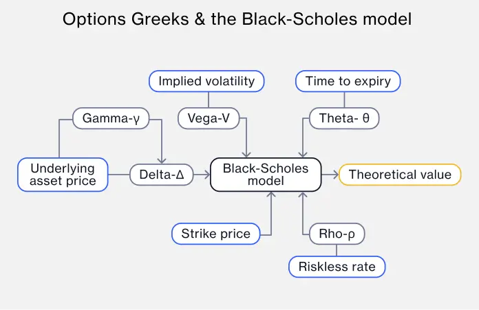
The Greeks are a set of metrics that describe these sensitivities. Among them, Gamma measures how fast Delta (the sensitivity of the option price to the underlying price) changes as the underlying price itself changes. So, how to calculate gamma?

In this article, we’ll focus on deriving the Gamma of a European option under the Black-Scholes model and implementing its calculation in C++. Whether you’re building a pricing engine or refining a hedging strategy, Gamma plays a key role in capturing the curvature of your position’s risk profile.

1. What is Gamma?

Gamma is one of the key Greeks in options trading. It measures the rate of change of Delta with respect to changes in the underlying asset price.

In other words:

• Delta tells you how much the option price changes when the underlying asset moves by a small amount.
• Gamma tells you how much Delta itself changes when the underlying price moves.

Interpretation:

• High Gamma means Delta is very sensitive to price changes — common for near-the-money options with short time to expiry.
• Low Gamma indicates Delta is more stable — typical for deep in-the-money or far out-of-the-money options.

2. The Gamma Formula

In the context of options pricing, Gamma arises naturally from the Black-Scholes Partial Differential Equation, which describes how the value of an option V(S,t) evolves with respect to the underlying asset price S and time t:

[math]\Large \frac{\partial V}{\partial t} + \frac{1}{2} \sigma^2 S^2 \frac{\partial^2 V}{\partial S^2} + r S \frac{\partial V}{\partial S} – r V = 0[/math]

In this equation:

• [math]\frac{\partial V}{\partial S}[/math] is Delta
• [math]\frac{\partial^2 V}{\partial S^2}[/math] is Gamma
• [math]r[/math] is the risk-free rate
• [math]\sigma[/math] is the volatility

From the Black-Scholes PDE, we isolate Gamma as the second derivative of the option value with respect to the underlying price. Under the Black-Scholes model, the closed-form expression for Gamma is:

[math]\Large \Gamma = \frac{N'(d_1)}{S \cdot \sigma \cdot \sqrt{T}}[/math]

Where:

• [math]N'(d_1)[/math] is the standard normal probability density at [math]d_1[/math]
• [math]S[/math] is the spot price of the underlying asset
• [math]\sigma[/math] is the volatility
• [math]T[/math] is the time to expiration

To derive the closed-form for Gamma, we start from the Black-Scholes formula for the price of a European call option:

[math]\Large C = S N(d_1) – K e^{-rT} N(d_2)[/math]

Here, the dependence on the spot price [math]S[/math] is explicit in both [math]S N(d_1)[/math] and [math]d_1[/math] itself, which is a function of [math]S[/math]:

[math]\Large d_1 = \frac{\ln(S/K) + (r + \frac{1}{2} \sigma^2)T}{\sigma \sqrt{T}}[/math]

To compute Gamma, we take the second partial derivative of [math]C[/math] with respect to [math]S[/math]. This involves applying the chain rule twice due to [math]d_1[/math]’s dependence on [math]S[/math].

After simplification (and canceling terms involving [math]d_2[/math]), what remains is:

[math]\Large \Gamma = \frac{N'(d_1)}{S \cdot \sigma \cdot \sqrt{T}}[/math]

This elegant result shows that Gamma depends only on the standard normal density at [math]d_1[/math], scaled by spot price, volatility, and time.

3. Implementation in Vanilla C++

Now that we’ve derived the closed-form formula for Gamma, let’s implement it in C++. The following code calculates the Gamma of a European option using the Black-Scholes model. It includes:

• A helper to compute the standard normal PDF
• A function to compute d1d_1d1​
• A gamma function implementing the formula
• A main() function that runs an example with sample inputs

Here’s the complete implementation to calculate gamma:

#include <iostream>
#include <cmath>

// Standard normal probability density function
double norm_pdf(double x) {
    return (1.0 / std::sqrt(2 * M_PI)) * std::exp(-0.5 * x * x);
}

// Compute d1 used in the Black-Scholes formula
double compute_d1(double S, double K, double r, double sigma, double T) {
    return (std::log(S / K) + (r + 0.5 * sigma * sigma) * T) / (sigma * std::sqrt(T));
}

// Compute Gamma using the closed-form Black-Scholes formula
double gamma(double S, double K, double r, double sigma, double T) {
    double d1 = compute_d1(S, K, r, sigma, T);
    return norm_pdf(d1) / (S * sigma * std::sqrt(T));
}

int main() {
    double S = 100.0;     // Spot price
    double K = 100.0;     // Strike price
    double r = 0.05;      // Risk-free interest rate
    double sigma = 0.2;   // Volatility
    double T = 1.0;       // Time to maturity in years

    double gamma_val = gamma(S, K, r, sigma, T);
    std::cout << "Gamma: " << gamma_val << std::endl;

    return 0;
}

After compilation, running the executable will calculate gamma:

➜  build ./gamma        
Gamma: 0.018762

Code of the article with Readme for compilation and execution:

https://github.com/cppforquants/gamma/tree/main

Traders and risk managers rely on accurate values for Delta, Gamma, Vega, and other Greeks to hedge portfolios and manage exposure. Today, we’re going to see how to use automatic differentiation for greeks calculation.

Traditionally, these sensitivities are calculated using finite difference methods, which approximate derivatives numerically. While easy to implement, this approach suffers from trade-offs between precision, performance, and stability. Enter Automatic Differentiation (AD): a modern technique that computes derivatives with machine precision and efficient performance.

In this article, we explore how to compute Greeks using automatic differentiation in C++ using the lightweight AD library Adept.

1. Background: Greeks and Finite Differences

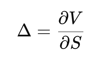
The Delta of a derivative is the rate of change of its price with respect to the underlying asset price:

[math] \Large {\Delta = \displaystyle \frac{\partial V}{\partial S}} [/math]

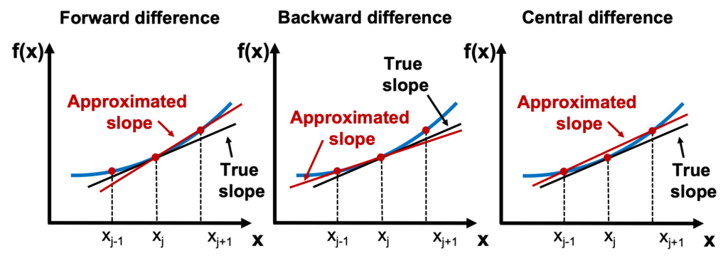
With finite differences, we might compute:

[math] \Large { \Delta \approx \frac{V(S + \epsilon) – V(S)}{\epsilon} } [/math]

This introduces:

• Truncation error if ε is too large,
• Rounding error if ε is too small,
• And 2N evaluations for N Greeks.

2. Automatic Differentiation: Another Way

Automatic Differentiation (AD) is a technique for computing exact derivatives of functions expressed as computer programs. It is not the same as:

• Numerical differentiation (e.g., finite differences), which approximates derivatives and is prone to rounding/truncation errors.
• Symbolic differentiation (like in computer algebra systems), which manipulates expressions analytically but can become unwieldy and inefficient.

AD instead works by decomposing functions into elementary operations and systematically applying the chain rule to compute derivatives alongside function evaluation.

🔄 How It Works

1. Operator Overloading (in C++)
   AD libraries in C++ (like Adept or CppAD) define a custom numeric type—say, adouble—which wraps a real number and tracks how it was computed. Arithmetic operations (+, *, sin, exp, etc.) are overloaded to record both the value and the derivative.
2. Taping
   During function execution, the AD library records (“tapes”) every elementary operation (e.g., x * y, log(x), etc.) into a computational graph. Each node stores the local derivative of the output with respect to its inputs.
3. Chain Rule Application
   Once the function is evaluated, AD applies the chain rule through the computational graph to compute the final derivatives.
   • Forward mode AD: computes derivatives with respect to one or more inputs.
   • Reverse mode AD: computes derivatives of one output with respect to many inputs (more efficient for scalar-valued functions with many inputs, like in ML or risk models).

🎯 Why It’s Powerful

• Exact to machine precision (unlike finite differences)
• Fast and efficient: typically only 5–10x the cost of the original function
• Compositional: works on any function composed of differentiable primitives, no matter how complex

📦 In C++ Quant Contexts

AD shines in quant applications where:

• Analytical derivatives are difficult to compute or unavailable (e.g., path-dependent or exotic derivatives),
• Speed and accuracy matter (e.g., calibration loops or sensitivity surfaces),
• You want to avoid hard-coding Greeks and re-deriving math manually.

3. C++ Implementation Using CppAD

Install CppAD and link it with your C++ project:

git clone https://github.com/coin-or/CppAD.git
cd CppAD
mkdir build
cd build
cmake ..
make
make install

Then link the library to your CMakeLists.txt:

cmake_minimum_required(VERSION 3.10)
project(CppADGreeks)

set(CMAKE_CXX_STANDARD 17)

# Find and link CppAD
find_path(CPPAD_INCLUDE_DIR cppad/cppad.hpp PATHS /usr/local/include)
find_library(CPPAD_LIBRARY NAMES cppad_lib PATHS /usr/local/lib)

if (NOT CPPAD_INCLUDE_DIR OR NOT CPPAD_LIBRARY)
    message(FATAL_ERROR "CppAD not found")
endif()

include_directories(${CPPAD_INCLUDE_DIR})
link_libraries(${CPPAD_LIBRARY})

# Example executable
add_executable(automaticdiff ../automaticdiff.cpp)
target_link_libraries(automaticdiff ${CPPAD_LIBRARY})

And the following code is in my automaticdiff.cpp:

#include <cppad/cppad.hpp>
#include <iostream>
#include <vector>
#include <cmath>

template <typename T>
T norm_cdf(const T& x) {
    return 0.5 * CppAD::erfc(-x / std::sqrt(2.0));
}

int main() {
    using CppAD::AD;

    std::vector<AD<double>> X(1);
    X[0] = 105.0;  // Spot price

    CppAD::Independent(X);

    double K = 100.0, r = 0.05, sigma = 0.2, T = 1.0;
    AD<double> S = X[0];

    AD<double> d1 = (CppAD::log(S / K) + (r + 0.5 * sigma * sigma) * T) / (sigma * std::sqrt(T));
    AD<double> d2 = d1 - sigma * std::sqrt(T);

    AD<double> price = S * norm_cdf(d1) - K * CppAD::exp(-r * T) * norm_cdf(d2);

    std::vector<AD<double>> Y(1);
    Y[0] = price;

    CppAD::ADFun<double> f(X, Y);

    std::vector<double> x = {105.0};
    std::vector<double> delta = f.Jacobian(x);

    std::cout << "Call Price: " << CppAD::Value(price) << std::endl;
    std::cout << "Delta (∂Price/∂S): " << delta[0] << std::endl;

    return 0;
}

After compiling and running this code, we get a delta:

➜  build ./automaticdiff
Call Price: 13.8579
Delta (∂Price/∂S): 0.723727

4. Explanation of the Code

Here’s the key part of the code again:

cppCopierModifierstd::vector<AD<double>> X(1);
X[0] = 105.0;  // Spot price S
CppAD::Independent(X);       // Start taping operations

// Constants
double K = 100.0, r = 0.05, sigma = 0.2, T = 1.0;
AD<double> S = X[0];

// Black-Scholes price formula
AD<double> d1 = (CppAD::log(S / K) + (r + 0.5 * sigma * sigma) * T) / (sigma * std::sqrt(T));
AD<double> d2 = d1 - sigma * std::sqrt(T);
AD<double> price = S * norm_cdf(d1) - K * CppAD::exp(-r * T) * norm_cdf(d2);

std::vector<AD<double>> Y(1); Y[0] = price;
CppAD::ADFun<double> f(X, Y);  // Create a differentiable function f: S ↦ price

std::vector<double> x = {105.0};
std::vector<double> delta = f.Jacobian(x);  // Get ∂price/∂S

✅ What This Code Does (Conceptually)

Step 1 – You Define a Function:

The code defines a function f(S) = Black-Scholes call price as a function of spot S. But unlike normal code, you define this using AD types (AD<double>), so CppAD can trace the computation.

Step 2 – CppAD Records All Operations:

When you run this line:

CppAD::Independent(X);

CppAD starts building a computational graph. Every operation you do on S (which is X[0]) is recorded:

• log(S / K)
• d1
• d2
• norm_cdf(d1)
• …
• final result price

This is like taping a math program:
CppAD now knows how the output (price) was built from the input (S).

Step 3 – You “seal” the function:

CppAD::ADFun<double> f(X, Y);

This finalizes the tape into a function:

[math] \Large{f: S \mapsto \text{price}} [/math]

🤖 How AD Gets the Derivative

Using:

std::vector<double> delta = f.Jacobian(x);

CppAD:

• Evaluates the forward pass to get intermediate values (just like normal code),
• Then walks backward through the graph, applying the chain rule at each node to compute:

[math] \Large{ \Delta = \frac{\partial \text{price}}{\partial S} } [/math]

This is the exact derivative, not an approximation.

⚙️ Summary: How the Code Avoids Finite Difference Pitfalls

Delta is one of the most important Greeks in options pricing. It measures how sensitive an option’s price is to changes in the price of the underlying asset. How to perform a delta calculation? Let’s derive and it and calculate it in C++.

1. Derive the Delta Formula for a Call Option

Delta is defined as the rate of change of an option’s price with respect to changes in the underlying asset price. In mathematical terms, it’s the first partial derivative of the option value V with respect to the underlying asset price S:

[math] \Large{\Delta = \frac{\partial V}{\partial S}} [/math]

Under the Black-Scholes framework, the price of a European call option is given by:

[math]\Large{C = S N(d_1) – K e^{-rT} N(d_2)}[/math]

Where:

• S is the current spot price of the underlying
• K is the strike price
• r is the risk-free interest rate
• T is the time to maturity
• N(⋅) is the cumulative distribution function of the standard normal distribution
• [math]d_1 = \frac{\ln(S/K) + \left(r + \frac{\sigma^2}{2} \right) T}{\sigma \sqrt{T}}[/math]
• [math]d_2 = d_1 – \sigma \sqrt{T}[/math]

To compute the Delta of a call option, we differentiate the Black-Scholes formula with respect to S:

[math]\Large \frac{\partial C}{\partial S} = \frac{\partial}{\partial S} \left[ S N(d_1) – K e^{-rT} N(d_2) \right][/math]

Only the first term depends on S directly. The derivative of the first term requires the chain rule, since d1​ is a function of S as well. Thus:

[math]\Large \frac{\partial C}{\partial S} = N(d_1)[/math]

Therefore, the Delta of a European call option is:

[math]\Large \Delta_{\text{call}} = N(d_1)[/math]

2. Derive the Delta Formula For a Put Option

For a put option, we apply the same steps to the Black-Scholes formula for puts:

[math]\Large P = K e^{-rT} N(-d_2) – S N(-d_1)[/math]

Where:

• S is the current spot price of the underlying
• K is the strike price
• r is the risk-free interest rate
• T is the time to maturity
• N(⋅) is the cumulative distribution function of the standard normal distribution
• [math]d_1 = \frac{\ln(S/K) + \left(r + \frac{\sigma^2}{2} \right) T}{\sigma \sqrt{T}}[/math]
• [math]d_2 = d_1 – \sigma \sqrt{T}[/math]

Differentiating:

[math]\Large \frac{\partial P}{\partial S} = -N(-d_1) = N(d_1) – 1[/math]

Hence, the Delta of a European put option is:

[math]\Large \Delta_{\text{put}} = N(d_1) – 1[/math]

3. Delta Calculation in C++ Without Library

We can simply implement the recipes above to calculate delta call and delta put:

#include <cmath>
#include <iostream>

// Cumulative normal distribution function
double norm_cdf(double x) {
    return 0.5 * std::erfc(-x / std::sqrt(2));
}

double black_scholes_delta(
    bool is_call,
    double S,     // Spot
    double K,     // Strike
    double T,     // Time to maturity
    double r,     // Risk-free rate
    double sigma  // Volatility
) {
    double d1 = (std::log(S / K) + (r + 0.5 * sigma * sigma) * T)
                / (sigma * std::sqrt(T));

    if (is_call) {
        return norm_cdf(d1);
    } else {
        return norm_cdf(d1) - 1.0;
    }
}

Then:

int main() {
    double S = 100.0;
    double K = 100.0;
    double T = 1.0;
    double r = 0.05;
    double sigma = 0.2;

    double delta_call = black_scholes_delta(true, S, K, T, r, sigma);
    double delta_put  = black_scholes_delta(false, S, K, T, r, sigma);

    std::cout << "Call Delta: " << delta_call << std::endl;
    std::cout << "Put Delta: "  << delta_put  << std::endl;
    return 0;
}

This is implements the analytical formula for Delta explicitly. It’s lightweight and very fast, great for educational or performance-critical code. It assumes flat rates and no dividends.

But what if you want something less generic?

4. Delta Calculation in C++ With Quantlib

Well, we can use the bazooka:

#include <ql/quantlib.hpp>
#include <iostream>

using namespace QuantLib;

int main() {
    Calendar calendar = TARGET();
    Date today(23, June, 2025);
    Settings::instance().evaluationDate() = today;

    // Common option parameters
    Real underlying = 100.0;
    Real strike = 100.0;
    Spread dividendYield = 0.0;
    Rate riskFreeRate = 0.05;
    Volatility volatility = 0.20;
    Date maturity = today + Period(1, Years);
    DayCounter dayCounter = Actual365Fixed();

    // Market data handles
    Handle<Quote> underlyingH(boost::shared_ptr<Quote>(new SimpleQuote(underlying)));
    Handle<YieldTermStructure> flatDividendTS(boost::shared_ptr<YieldTermStructure>(
        new FlatForward(today, dividendYield, dayCounter)));
    Handle<YieldTermStructure> flatRiskFreeTS(boost::shared_ptr<YieldTermStructure>(
        new FlatForward(today, riskFreeRate, dayCounter)));
    Handle<BlackVolTermStructure> flatVolTS(boost::shared_ptr<BlackVolTermStructure>(
        new BlackConstantVol(today, calendar, volatility, dayCounter)));

    boost::shared_ptr<BlackScholesMertonProcess> bsmProcess(
        new BlackScholesMertonProcess(underlyingH, flatDividendTS, flatRiskFreeTS, flatVolTS));

    // Loop over Call and Put options
    for (auto type : {Option::Call, Option::Put}) {
        std::string typeStr = (type == Option::Call ? "Call" : "Put");

        boost::shared_ptr<StrikedTypePayoff> payoff(new PlainVanillaPayoff(type, strike));
        boost::shared_ptr<Exercise> exercise(new EuropeanExercise(maturity));
        VanillaOption option(payoff, exercise);

        option.setPricingEngine(boost::shared_ptr<PricingEngine>(
            new AnalyticEuropeanEngine(bsmProcess)));

        std::cout << typeStr << " Delta: " << option.delta() << std::endl;
    }

    return 0;
}

✅ The QuantLib implementation:

• Wraps the same math, but within a complete pricing engine (AnalyticEuropeanEngine).
• Uses market objects like Quote, YieldTermStructure, and BlackVolTermStructure, which can evolve over time.
• Supports dividends, yield curves, non-constant volatility, and more.

In a word, it’s heavier but more flexible and extensible, making it better suited for production systems or derivatives desks.

5. Let’s Run Both and Compare?

Let’s start with the first version, after compiling and running:

➜  ./delta_vanilla                                                              
Call Delta: 0.636831
Put Delta: -0.363169

Now, the Quantlib version:

➜  build ./delta_quantlib 
Call Delta: 0.636831
Put Delta: -0.363169

The exact same!

What about execution time?

For the first version, it’s instant, <<0.01s:

➜  build time ./delta_vanilla 

./delta_vanilla  0.00s user 0.00s

For the Quantlib version, ~0.01s, slightly slower:

➜  build time ./delta_quantlib

./delta_quantlib  0.00s user 0.01s

4. Summarize Both Implementations for Delta Calculation

If you’re writing an educational article or prototyping, the vanilla version is perfect. If you’re integrating with a full market data and pricing system, QuantLib is the go-to.

Code of the article with Readme for compilation and execution:

https://github.com/cppforquants/delta/tree/main