Volatility

Implied volatility isn’t flat across strikes: it curves. It’s like a smile: the volatility smile.

When plotted against strike price, implied volatilities for call options typically form a smile, with lower volatilities near-the-money and higher volatilities deep in- or out-of-the-money. This shape reflects real-world market dynamics, like the increased demand for tail-risk protection and limitations of the Black-Scholes model.

In this article, we’ll implement a simple C++ tool to compute this volatility smile from observed market prices, helping us visualize and understand its structure.

1. What’s a Volatility Smile?

A volatility smile is a pattern observed in options markets where implied volatility (IV) is not constant across different strike prices — contrary to what the Black-Scholes model assumes. When plotted (strike on the x-axis, IV on the y-axis), the graph forms a smile-shaped curve.

• At-the-money (ATM) options tend to have the lowest implied volatility.
• In-the-money (ITM) and out-of-the-money (OTM) options show higher implied volatility.

If you plot IV vs. strike price, the shape curves upward at both ends, resembling a smile.

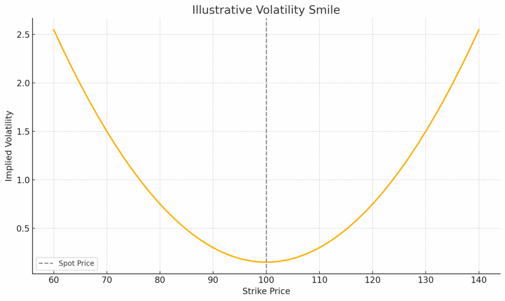
Implied volatility is lowest near the at-the-money (ATM) strike and increases for both in-the-money (ITM) and out-of-the-money (OTM) options.

This convex shape reflects typical market observations and diverges from the flat IV assumption in Black-Scholes.

For call options, the left side of the volatility smile (low strikes) is in-the-money, the center is at-the-money, and the right side (high strikes) is out-of-the-money.

2. In-the-money (ITM), At-the-money (ATM), Out-of-the-money (OTM)

These terms describe the moneyness of an option:

• ITM: Has intrinsic value — profitable if exercised now.
• ATM: Strike is close to spot price — most sensitive to volatility (highest gamma).
• OTM: No intrinsic value — only time value.

Here are two quick scenarios:

In-the-Money (ITM) Call – Profitable Scenario:

A trader buys a call option with a strike price of £90 when the stock is at £95 (already ITM).
Later, the stock rises to £105, and the option gains intrinsic value.
🔁 Trader profits by exercising the option or selling it for more than they paid.

Out-of-the-Money (OTM) Call – Profitable Scenario:

A trader buys a call option with a strike price of £110 when the stock is at £100 (OTM, cheaper).
Later, the stock jumps to £120, making the option now worth at least £10 intrinsic.
🔁 Trader profits from the big move, even though the option started OTM.

3. Why this pattern?

The volatility smile arises because market participants do not believe asset returns follow a perfect normal distribution. Instead, they expect more frequent extreme moves in either direction, what statisticians call “fat tails.” To account for this, traders are willing to pay more for options that are far out-of-the-money or deep in-the-money, especially since these positions offer outsized payoffs in rare but impactful events. This increased demand pushes up the implied volatility for these strikes.

Moreover, options at the tails often serve as hedging tools.

• For example, portfolio managers commonly buy far out-of-the-money puts to protect against a market crash. Similarly, speculative traders might buy cheap out-of-the-money calls hoping for a large upward movement. This consistent demand at the tails drives up their prices, and consequently, their implied volatilities.

• In contrast, at-the-money options are more frequently traded and are typically the most liquid. Because their strike price is close to the current market price, they tend to reflect the market’s consensus on future volatility more accurately. There’s less uncertainty and speculation around them, and they don’t carry the same kind of tail risk premium.

As a result, the implied volatility at the money tends to be lower, forming the bottom of the volatility smile.

4. Implementation in C++

Here is an implementation in C++ using Black-Scholes:

#include <iostream>
#include <cmath>
#include <vector>
#include <iomanip>

// Black-Scholes formula for a European call option
double black_scholes_call(double S, double K, double T, double r, double sigma) {
    double d1 = (std::log(S / K) + (r + 0.5 * sigma * sigma) * T) / (sigma * std::sqrt(T));
    double d2 = d1 - sigma * std::sqrt(T);

    auto N = [](double x) {
        return 0.5 * std::erfc(-x / std::sqrt(2));
    };

    return S * N(d1) - K * std::exp(-r * T) * N(d2);
}

// Bisection method to compute implied volatility
double implied_volatility(double market_price, double S, double K, double T, double r,
                          double tol = 1e-5, int max_iter = 100) {
    double low = 0.0001;
    double high = 2.0;

    for (int i = 0; i < max_iter; ++i) {
        double mid = (low + high) / 2.0;
        double price = black_scholes_call(S, K, T, r, mid);

        if (std::abs(price - market_price) < tol) return mid;
        if (price > market_price) high = mid;
        else low = mid;
    }

    return (low + high) / 2.0; // best guess
}

// Synthetic volatility smile to simulate market prices
double synthetic_volatility(double K, double S) {
    double base_vol = 0.15;
    return base_vol + 0.0015 * std::pow(K - S, 2);
}

int main() {
    double S = 100.0;     // Spot price
    double T = 0.5;       // Time to maturity in years
    double r = 0.01;      // Risk-free rate

    std::cout << "Strike\tMarketPrice\tImpliedVol\n";

    for (double K = 60; K <= 140; K += 2.0) {
        double true_vol = synthetic_volatility(K, S);
        double market_price = black_scholes_call(S, K, T, r, true_vol);
        double iv = implied_volatility(market_price, S, K, T, r);

        std::cout << std::fixed << std::setprecision(2)
                  << K << "\t" << market_price << "\t\t" << std::setprecision(4) << iv << "\n";
    }

    return 0;
}

We aim to simulate and visualize a volatility smile by:

1. Generating synthetic market prices for European call options using a non-constant volatility function.
2. Computing the implied volatility by inverting the Black-Scholes model using a bisection method.
3. Printing the results to observe how implied volatility varies across strike prices.
   

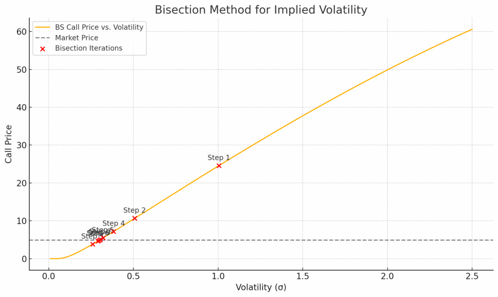
We compute implied volatility by numerically inverting the Black-Scholes formula:

double implied_volatility(double market_price, double S, double K, double T, double r)

We seek the value of [math]\sigma[/math] such that:

[math] C_{\text{BS}}(S, K, T, r, \sigma) \approx \text{Market Price} [/math]

We use the bisection method, iteratively narrowing the interval [math][\sigma_{\text{low}}, \sigma_{\text{high}}][/math] until the difference between the model price and the market price is within a small tolerance.

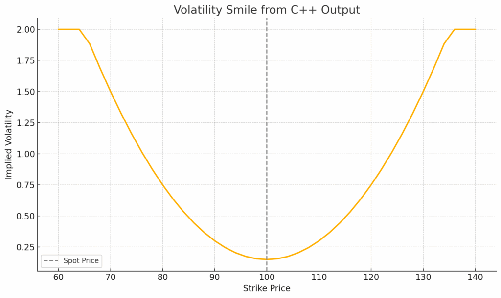
Now, here is the plot of your volatility smile using the output from the C++ program.

After compiling our code:

mkdir build
cd build
cmake ..
make

We can run it:

./volatilitysmile

And get:

Strike  MarketPrice     ImpliedVol
60.00   72.18           2.0000
62.00   68.21           2.0000
64.00   64.09           2.0000
66.00   59.85           1.8840
68.00   55.55           1.6860
70.00   51.23           1.5000
72.00   46.92           1.3260
74.00   42.68           1.1640
76.00   38.53           1.0140
78.00   34.51           0.8760
80.00   30.64           0.7500
82.00   26.95           0.6360
84.00   23.45           0.5340
86.00   20.17           0.4440
88.00   17.11           0.3660
90.00   14.28           0.3000
92.00   11.70           0.2460
94.00   9.38            0.2040
96.00   7.36            0.1740
98.00   5.70            0.1560
100.00  4.47            0.1500
102.00  3.73            0.1560
104.00  3.44            0.1740
106.00  3.57            0.2040
108.00  4.06            0.2460
110.00  4.91            0.3000
112.00  6.10            0.3660
114.00  7.64            0.4440
116.00  9.55            0.5340
118.00  11.83           0.6360
120.00  14.48           0.7500
122.00  17.49           0.8760
124.00  20.86           1.0140
126.00  24.57           1.1640
128.00  28.59           1.3260
130.00  32.89           1.5000
132.00  37.44           1.6860
134.00  42.19           1.8840
136.00  47.07           2.0000
138.00  52.03           2.0000
140.00  57.01           2.0000

As expected, implied volatility is lowest near the at-the-money strike (100) and rises symmetrically for deep in-the-money and out-of-the-money strikes forming the characteristic smile shape:

The code for this article is accessible here:

https://github.com/cppforquants/volatilitysmile

Volatility is a cornerstone concept in finance, used to measure the degree of variation in the price of a financial instrument. Two of the most commonly referenced types are Implied Volatility (IV) and Historical Volatility (HV), and while they both aim to assess risk, they do so from different perspectives.

Implied Volatility is forward-looking. Derived from option prices using models like Black-Scholes, it reflects the market’s expectations of future price movement. Higher IV typically signals greater anticipated risk or uncertainty.

HV is objective and purely data-driven, while IV incorporates market sentiment and supply-demand dynamics in the options market.

1. Derive Black-Scholes PDE Solution for European Call Options

To derive implied volatility from the Black-Scholes model, you’re essentially trying to find the volatility (σ) that, when plugged into the Black-Scholes formula, yields the market price of the option.

Let’s start from Black-Scholes.

[math]
\Large{dS_t = \mu S_t \, dt + \sigma S_t \, dW_t}
[/math]

is a stochastic differential equation (SDE) — it’s the core model behind how asset prices evolve over time in the Black-Scholes framework.

🔍 Term-by-Term Breakdown

The formula models price changes as having two components:

A deterministic part:

[math] \Large{\mu S_t \, dt} [/math]

This is the trend — the predictable, average growth over time.

A stochastic part:

[math] \Large{\sigma S_t \, dW_t} [/math]

This is the randomness — the noise or uncertainty in price movements.

• [math] \sigma [/math] scales the size of the randomness.
• [math] dW_t​ [/math] brings in randomness from a standard Brownian motion: the mean is 0 and the variance is dt

A first thing to do to reach the implied volatility question is to notice that to price options, we don’t use [math] mu [/math] because investors care about risk-adjusted returns.

Instead, we use r for the risk-neutral measure [math] \mathbb{Q} [/math], where:

[math] \Large{dS_t = r S_t \, dt + \sigma S_t \, dW_t^{\mathbb{Q}}} [/math]

• The drift becomes r, the risk-free rate.
• The randomness remains via [math] \sigma [/math] and [math] dW_t [/math]

🔍 Let’s define the call option price

[math]\Large{ C(t,S_t​)=price of a call option} [/math]

After a bit of work that we will not do in this article, we can derive the Black-Scholes PDE:

[math] \Large{\frac{\partial C}{\partial t} + r S_t \frac{\partial C}{\partial S} + \frac{1}{2} \sigma^2 S_t^2 \frac{\partial^2 C}{\partial S^2} – r C = 0} [/math]

Solving this PDE with the terminal condition:

[math] \Large{C(T, S_T) = \max(S_T – K, 0)} [/math]

gives us the option price at time t=0:

[math] \Large{C(\sigma) = S_0 \Phi(d_1) – K e^{-rT} \Phi(d_2)} [/math]

where:

[math] \Large{d_1 = \frac{\ln(S_0 / K) + (r + \frac{1}{2} \sigma^2) T}{\sigma \sqrt{T}}} [/math]

And

[math] \Large{d_2 = d_1 – \sigma \sqrt{T}} [/math]

2. Determine the Equation to Solve to get the Implied Volatility

We now take the market-observed option price [math] C_{market} [/math] and ask:

“What value of [math] \sigma [/math] makes the Black-Scholes price equal the market price?”

So we define the equation to solve:

[math] \Large{f(\sigma) = C(\sigma) \, – C_{\text{market}} = 0} [/math]

Since C(σ)C(\sigma)C(σ) involves Φ(d1)\Phi(d_1)Φ(d1​) and d1d_1d1​ contains σ\sigmaσ both in the numerator and denominator, there is no closed-form algebraic solution.

We solve it using numerical methods:

• Brent’s method (robust)
• Newton-Raphson (faster, requires Vega)
• Bisection (simple, slower)

What does it mean to solve that equation in a real-world context?

🧮 Example

Let’s say the following is true today:

👇 Now We Need To Solve:

[math] \Large{f(\sigma) = C(\sigma) – 2.50 = 0} [/math]

You plug different values of [math] \sigma [/math] into the Black-Scholes formula:

[math] \Large{C(\sigma) = S_0 \Phi(d_1) – K e^{-rT} \Phi(d_2)} [/math]

where:

[math] \Large{d_1 = \frac{\ln(S_0 / K) + (r + \frac{1}{2} \sigma^2) T}{\sigma \sqrt{T}}} [/math]

[math] \Large{d_2 = d_1 – \sigma \sqrt{T}} [/math]

And iterate until:

[math] \Large{C(\sigma) \approx 2.50} [/math].

So, how do we iterate to solve the volatility equation?

3. Use Quantlib to Solve the Implied Volatility Equation

Quantlib will solve that equation with a numerical method.

Here is the code for the example above:

#include <ql/quantlib.hpp>
#include <iostream>

using namespace QuantLib;

int main() {
    Calendar calendar = TARGET();
    Date today = Date::todaysDate();
    Settings::instance().evaluationDate() = today;

    // Option parameters
    Option::Type optionType = Option::Call;
    Real underlying = 100.0;
    Real strike = 105.0;
    Rate riskFreeRate = 0.05;
    Volatility initialVol = 0.20; // Just an initial guess
    Date maturity = calendar.advance(today, Period(30, Days));  // 30-day maturity
    Real marketPrice = 2.50;

    DayCounter dayCounter = Actual365Fixed();
    Handle<Quote> underlyingH(boost::shared_ptr<Quote>(new SimpleQuote(underlying)));

    // Constructing the yield curve and flat volatility surface
    Handle<YieldTermStructure> flatTermStructure(
        boost::shared_ptr<YieldTermStructure>(
            new FlatForward(today, riskFreeRate, dayCounter)));

    Handle<BlackVolTermStructure> flatVolTS(
        boost::shared_ptr<BlackVolTermStructure>(
            new BlackConstantVol(today, calendar, initialVol, dayCounter)));

    boost::shared_ptr<StrikedTypePayoff> payoff(
        new PlainVanillaPayoff(optionType, strike));

    boost::shared_ptr<Exercise> exercise(
        new EuropeanExercise(maturity));

    EuropeanOption option(payoff, exercise);

    Handle<YieldTermStructure> flatDividendTS(
    boost::shared_ptr<YieldTermStructure>(
        new FlatForward(today, 0.0, dayCounter)));

    boost::shared_ptr<BlackScholesMertonProcess> bsmProcess(
        new BlackScholesMertonProcess(underlyingH, 
                                      flatDividendTS, 
                                      flatTermStructure, 
                                      flatVolTS));

    // Calculate implied volatility
    try {
        Volatility impliedVol = option.impliedVolatility(
            marketPrice, bsmProcess, 1e-6, 100, 0.0001, 4.0);
        std::cout << "Implied Volatility: " << impliedVol << std::endl;
    } catch (std::exception& e) {
        std::cerr << "Error calculating implied volatility: " << e.what() << std::endl;
    }

    return 0;
}

after:

brew install quantlib

and setting up your CMakeLists.txt:

cmake_minimum_required(VERSION 3.10)
project(QuantLibImpliedVolExample)

set(CMAKE_CXX_STANDARD 17)

find_package(PkgConfig REQUIRED)
pkg_check_modules(QUANTLIB REQUIRED QuantLib)

include_directories(${QUANTLIB_INCLUDE_DIRS})
link_directories(${QUANTLIB_LIBRARY_DIRS})

add_executable(implied_vol src/volatility.cpp)
target_link_libraries(implied_vol ${QUANTLIB_LIBRARIES})

and now you can compile:

mkdir build
cd build
cmake ..
make

Eventually, you can run the executable:

> ./implied_vol
Implied Volatility: 0.318886