How to Calculate Potential Future Exposure (PFE)?

In modern investment banking, managing counterparty credit risk has become just as important as pricing the trade itself. Every derivative contract, from a simple interest rate swap to a complex cross-currency structure, carries the risk that the counterparty might default before the trade matures. When that happens, what really matters isn’t today’s mark-to-market, but what the exposure could be at the moment of default. That’s where Potential Future Exposure comes in: what is the Potential Future Exposure? How to calculate the Potential Future Exposure (PFE)?

1. What is the Potential Future Exposure(PFE)?

PFE quantifies the worst-case exposure a bank could face at a given confidence level and future time horizon. It doesn’t ask “what’s the average exposure?”, but rather “what’s the exposure in the 95th percentile scenario, one year from now?”. This risk-focused lens makes PFE a cornerstone of credit risk measurement, capital allocation, and pricing.

Before talking about PFE, we need to talk about mark-to-market (MtM), exposure end Expected Exposure (EE).

At any future time t, the exposure of a derivative or portfolio to a counterparty is defined as the positive mark-to-market (MtM) value from the bank’s perspective:

[math]\large E(t) = \max(V(t), 0)[/math]

where

• [math]V(t)[/math] is the (random) value of the portfolio at time [math]t[/math],
• [math]E(t)[/math] is the exposure — it cannot be negative, because if [math]V(t) < 0[/math], the exposure is zero (the counterparty owes you nothing).

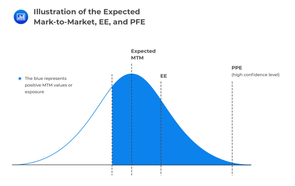
The Expected Exposure (EE) at time [math]t[/math] is the expected value of that random exposure across all simulated market scenarios:

[math]\large EE(t) = \mathbb{E}\big[ E(t) \big][/math]

It represents the average positive exposure at time [math]t[/math].

You can see it like this:

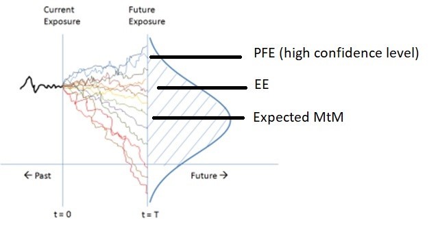
This other chart shows how a portfolio’s current exposure evolves into a distribution of possible future exposures, with the Expected MtM as the mean, the Expected Exposure (EE) as the average of positive values, and the Potential Future Exposure (PFE) marking the high-confidence tail (worst-case exposure) of that distribution.

For a given future time t and confidence level [math] \alpha [/math], the Potential Future Exposure (PFE) is defined as such:

• [math]E(t) = \max(V(t), 0)[/math] is the exposure,
• [math]V(t)[/math] is the mark-to-market value of the portfolio at time [math]t[/math], and
• [math]\alpha[/math] is the confidence level (e.g. 0.95 or 0.99).

we’re saying:

“Find the smallest value x such that the probability that exposure E(t) is below x is at least alpha.”

2. Why Does PFE Matter?

Potential Future Exposure (PFE) matters because it quantifies the worst-case credit exposure a bank could face with a counterparty at some point in the future. In essence, it asks: “How bad could it get?”

In trading, exposure today (the mark-to-market) is only a snapshot: what truly drives risk is how that exposure might evolve as markets move. PFE captures this by modeling thousands of potential future scenarios for rates, FX, equities, and credit spreads, and then measuring the high-percentile outcome (e.g. 95th or 99th).

Banks use PFE to set counterparty limits, ensuring that no single entity can cause unacceptable losses. Risk managers monitor these limits daily and reduce exposure through collateral, netting, or hedging.

PFE also feeds into regulatory capital frameworks such as Basel’s SA-CCR, influencing how much capital the bank must hold against derivative portfolios.

In trading desks, PFE affects pricing decisions: the higher the potential exposure, the higher the credit charge embedded in the trade price. Front-office, credit, and treasury teams all rely on PFE curves to understand how exposures behave over time and under stress.

In short, PFE transforms uncertain future risk into a measurable, actionable metric that connects market volatility, counterparty behavior, and balance-sheet safety — a critical pillar of counterparty credit risk management.

3. An Implementation in C++

Here’s a compact, production-style C++17 example that computes EE(t) and PFE(t, α) for a simple FX forward under GBM. It’s self-contained (only <random>, <vector>, etc.), and set up so you can swap in your own portfolio pricer later.

It simulates risk factor paths StS_tSt​, revalues the forward V(t)=N (St−K) DF(t)V(t)=N\,(S_t-K)\,DF(t)V(t)=N(St​−K)DF(t), takes exposure E(t)=max⁡(V(t),0)E(t)=\max(V(t),0)E(t)=max(V(t),0), then reports EE and PFE across a time grid.

// pfe_fx_forward.cpp
// C++17: Monte Carlo EE(t) and PFE(t, alpha) for an FX forward under GBM.

#include <algorithm>
#include <cmath>
#include <iomanip>
#include <iostream>
#include <numeric>
#include <random>
#include <string>
#include <vector>

// --------------------------- Utilities ---------------------------

// Quantile (0<alpha<1) of a vector (non-const because we sort).
double percentile(std::vector<double>& xs, double alpha) {
    if (xs.empty()) return 0.0;
    std::sort(xs.begin(), xs.end());
    // "linear interpolation between closest ranks" can be used;
    // here we do a simple nearest-rank with floor to be conservative for PFE.
    const double pos = alpha * (xs.size() - 1);
    const size_t idx = static_cast<size_t>(std::floor(pos));
    const double frac = pos - idx;
    if (idx + 1 < xs.size())
        return xs[idx] * (1.0 - frac) + xs[idx + 1] * frac;
    return xs.back();
}

// Discount factor assuming flat domestic rate r_d.
inline double discount(double r_d, double t) {
    return std::exp(-r_d * t);
}

// --------------------------- Model & Pricer ---------------------------

// Evolve FX under GBM: dS = S * ( (r_d - r_f) dt + sigma dW )
void simulate_paths_gbm(
    std::vector<std::vector<double>>& S, // [nPaths][nSteps+1]
    double S0, double r_d, double r_f, double sigma,
    double T, int nSteps, std::mt19937_64& rng)
{
    const double dt = T / nSteps;
    std::normal_distribution<double> Z(0.0, 1.0);

    for (size_t p = 0; p < S.size(); ++p) {
        S[p][0] = S0;
        for (int j = 1; j <= nSteps; ++j) {
            const double z = Z(rng);
            const double drift = (r_d - r_f - 0.5 * sigma * sigma) * dt;
            const double diff  = sigma * std::sqrt(dt) * z;
            S[p][j] = S[p][j - 1] * std::exp(drift + diff);
        }
    }
}

// Simple FX forward MtM from bank's perspective at time t:
// V(t) = N * ( S(t) - K ) * DF_d(t)
// (Domestic-discounted payoff; sign assumes receiving S, paying K at T.)
// If you want precise forward maturing at T, you can scale by DF(T)/DF(t)
// and/or set value only at maturity; here we keep a running MtM proxy.
inline double forward_mtm(double notional, double S_t, double K, double r_d, double t) {
    return notional * (S_t - K) * discount(r_d, t);
}

// Exposure is positive part of MtM.
inline double exposure(double Vt) { return std::max(Vt, 0.0); }

// --------------------------- Main EE/PFE Engine ---------------------------

struct Results {
    std::vector<double> times;     // size nSteps+1
    std::vector<double> EE;        // Expected Exposure at each time
    std::vector<double> PFE;       // Potential Future Exposure at each time
};

Results compute_EE_PFE_FXForward(
    int nPaths, int nSteps, double T,
    double S0, double r_d, double r_f, double sigma,
    double notional, double strikeK,
    double alpha, uint64_t seed = 42ULL)
{
    // 1) Simulate FX paths
    std::mt19937_64 rng(seed);
    std::vector<std::vector<double>> S(nPaths, std::vector<double>(nSteps + 1));
    simulate_paths_gbm(S, S0, r_d, r_f, sigma, T, nSteps, rng);

    // 2) Time grid
    std::vector<double> times(nSteps + 1);
    for (int j = 0; j <= nSteps; ++j) times[j] = (T * j) / nSteps;

    // 3) For each time, compute exposures across paths, then EE and PFE
    std::vector<double> EE(nSteps + 1, 0.0);
    std::vector<double> PFE(nSteps + 1, 0.0);
    std::vector<double> bucket(nPaths);

    for (int j = 0; j <= nSteps; ++j) {
        const double t = times[j];

        // Build exposure samples at time t across paths
        for (int p = 0; p < nPaths; ++p) {
            const double Vt = forward_mtm(notional, S[p][j], strikeK, r_d, t);
            bucket[p] = exposure(Vt);
        }

        // EE(t) = mean of positive exposures
        const double sum = std::accumulate(bucket.begin(), bucket.end(), 0.0);
        EE[j] = sum / static_cast<double>(nPaths);

        // PFE(t, alpha) = alpha-quantile of exposures
        // (we make a working copy because percentile sorts in-place)
        std::vector<double> tmp = bucket;
        PFE[j] = percentile(tmp, alpha);
    }

    return { std::move(times), std::move(EE), std::move(PFE) };
}

// --------------------------- Demo / CLI ---------------------------

int main(int argc, char** argv) {
    // Default parameters (override via argv if desired).
    int    nPaths  = 20000;
    int    nSteps  = 20;         // e.g., quarterly over 5 years => set T=5.0 and nSteps=20
    double T       = 2.0;        // years
    double S0      = 1.10;       // spot FX (e.g., USD per EUR)
    double r_d     = 0.035;      // domestic rate
    double r_f     = 0.015;      // foreign rate
    double sigma   = 0.12;       // FX vol
    double N       = 10'000'000; // notional
    double K       = 1.12;       // forward strike
    double alpha   = 0.95;       // PFE quantile
    uint64_t seed  = 42ULL;

    // (Optional) basic CLI parsing for quick tweaks
    if (argc > 1) nPaths = std::stoi(argv[1]);
    if (argc > 2) nSteps = std::stoi(argv[2]);
    if (argc > 3) T      = std::stod(argv[3]);

    auto res = compute_EE_PFE_FXForward(
        nPaths, nSteps, T, S0, r_d, r_f, sigma, N, K, alpha, seed
    );

    // Pretty print
    std::cout << std::fixed << std::setprecision(6);
    std::cout << "t,EE,PFE\n";
    for (size_t j = 0; j < res.times.size(); ++j) {
        std::cout << res.times[j] << "," << res.EE[j] << "," << res.PFE[j] << "\n";
    }

    // A quick sanity summary at T/2 and T
    auto halfway = res.times.size() / 2;
    std::cout << "\nSummary\n";
    std::cout << "EE(T/2)  = " << res.EE[halfway] << "\n";
    std::cout << "PFE(T/2) = " << res.PFE[halfway] << "\n";
    std::cout << "EE(T)    = " << res.EE.back() << "\n";
    std::cout << "PFE(T)   = " << res.PFE.back() << "\n";

    return 0;
}

3. Explanation of the Code

So, how to calculate the Pontential Future Exposure(PFE)? This C++ program demonstrates how to estimate Expected Exposure (EE) and Potential Future Exposure (PFE) using a simple Monte Carlo engine for an FX forward.

It begins by simulating many potential future FX rate paths under a Geometric Brownian Motion (GBM) model, where each path represents how the exchange rate might evolve given drift, volatility, and random shocks. For every time step, the program computes the mark-to-market (MtM) of the FX forward as the discounted notional times the difference between simulated spot and strike.

For every time step, the program computes the mark-to-market (MtM) of the FX forward as the discounted notional times the difference between simulated spot and strike. Negative MtM values imply the bank owes the counterparty, so exposures are floored at zero using max(Vt, 0). Across all paths, the program averages these exposures to get the Expected Exposure EE(t) and extracts the high-quantile value to obtain PFE(t, α): the 95th percentile exposure. It iterates this process across the time grid to build the full exposure profile. The simulation uses <random> for Gaussian draws, std::vector containers for efficiency, and a clean modular structure separating simulation, pricing, and analytics. Finally, results are printed as a CSV table of time, EE, and PFE, ready for plotting or integration into a larger risk system.

4. What are the key parameters driving the PFE value?

PFE is not a static number: it’s shaped by a mix of market dynamics, trade structure, and risk mitigation terms.
At its core, it reflects how volatile and directional the portfolio’s mark-to-market (MtM) could become under plausible future scenarios.
The main drivers are:

a. Market Volatility (σ)
The higher the volatility of the underlying risk factors (interest rates, FX, equities, credit spreads), the wider the future distribution of MtM values.
Since PFE is a high quantile of that distribution, higher volatility directly pushes PFE up.

b. Time Horizon (t)
Exposure uncertainty compounds over time.
The longer the time horizon, the more potential market moves accumulate, leading to a larger spread of outcomes and therefore higher PFE.

c. Product Type and Optionality
Linear products (like forwards or swaps) have exposures that evolve predictably, while nonlinear products (like options) exhibit asymmetric exposure.
For example, an option seller’s exposure can explode if volatility rises, so the product payoff shape strongly affects the PFE profile.

d. Counterparty Netting Set
If multiple trades exist under the same netting agreement, positive and negative MtMs offset each other.
A large, well-balanced netting set reduces overall exposure variance and therefore lowers PFE.

e. Collateralization / CSA Terms
Credit Support Annex (CSA) terms (thresholds, minimum transfer amounts, margin frequency): they determine how much exposure remains unsecured.
Frequent margining and low thresholds sharply reduce PFE; loose or infrequent margining increases it

f. Correlation and Wrong-Way Risk
If the exposure tends to rise when the counterparty’s credit worsens (e.g. a borrower correlated with its asset), this wrong-way risk amplifies effective PFE because losses are more likely when the counterparty defaults

g. Interest Rate Differentials and Discounting
In FX and IR products, differences between domestic and foreign rates (or curve shapes) affect the drift of MtM paths.
Higher discount rates reduce future MtMs and hence lower PFE in present-value terms

h. Confidence Level (α)
By definition, PFE depends on the percentile you choose: 95%, 97.5%, or 99%.
A higher confidence level means a deeper tail cut and therefore a higher PFE.