Best C++ Libraries for Quants: An Overview

C++ is widely used in quant finance for its speed and control. To build pricing engines, risk models, and simulations efficiently, quants rely on specific libraries. This article gives a quick overview of the most useful ones:

• QuantLib – derivatives pricing and fixed income
• Eigen – fast linear algebra
• Boost – utilities, math, random numbers
• NLopt – non-linear optimization

Each library is explained with use cases and code snippets: let’s discover the best C++ libraries for quants.

1. Quantlib: The Ultimate Quant Toolbox

QuantLib is an open-source C++ library for modeling, pricing, and managing financial instruments.
It was started in 2000 by Ferdinando Ametrano and later developed extensively by Luigi Ballabio, who remains one of its lead maintainers.

QuantLib is used by several major institutions and fintech firms. J.P. Morgan and Bank of America have referenced it in quant research roles and academic work. Bloomberg employs developers who have contributed to the library. OpenGamma, StatPro, and TriOptima have built tools on top of it. ING has published QuantLib-based projects on GitHub. It’s also used in academic settings like Oxford, ETH Zurich, and NYU for teaching quantitative finance. While not always publicly disclosed, QuantLib remains a quiet industry standard across banks, hedge funds, and research labs.

An example with Quantlib: Black-Scholes European call option pricing

This example calculates the fair price of a European call option using the Black-Scholes model. It sets up the option parameters, market conditions, and uses QuantLib’s analytic engine to compute the net present value (NPV) of the option.

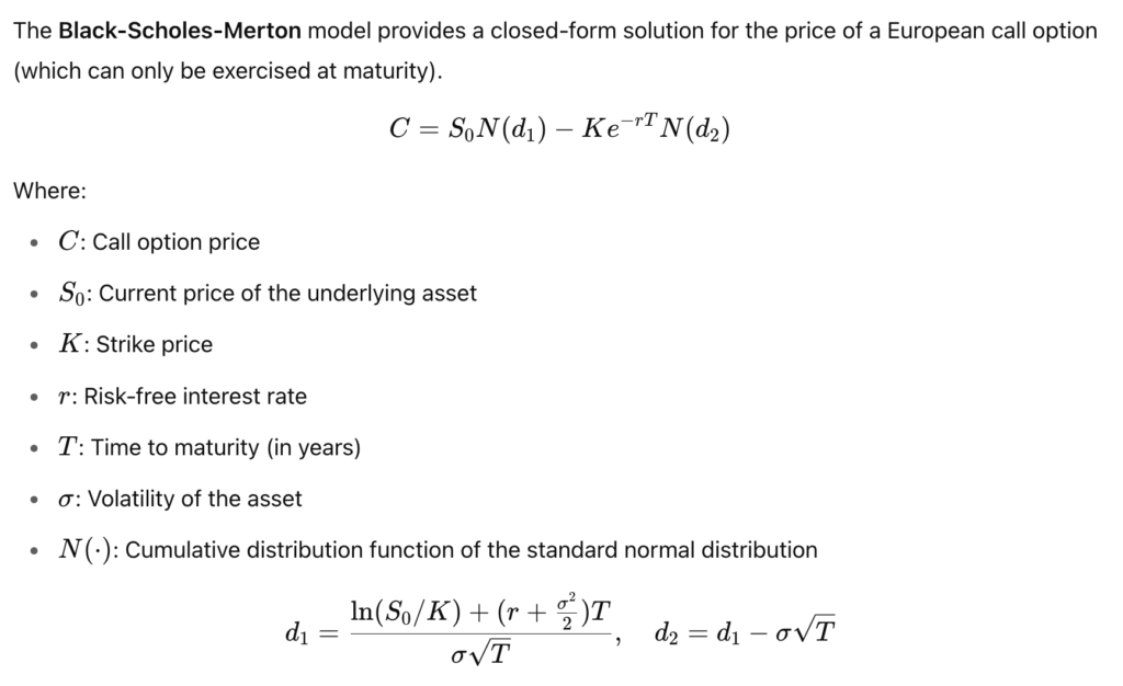
The Black-Scholes-Merton model provides a closed-form solution for the price of a European call option (which can only be exercised at maturity).

A call option is a financial contract that gives the buyer the right, but not the obligation, to buy an underlying asset (like a stock) at a specified strike price (K) on or before a specified maturity date (T).
The buyer pays a premium for this right. If the asset price STS_TST​ at maturity is higher than the strike price, the call is “in the money” and can be exercised for profit.

Let’s implement it with Quantlib:

#include <ql/quantlib.hpp>
#include <iostream>

int main() {
    using namespace QuantLib;

    Calendar calendar = TARGET();
    Date settlementDate(19, June, 2025);
    Settings::instance().evaluationDate() = settlementDate;

    // Option parameters
    Option::Type type(Option::Call);
    Real underlying = 100;
    Real strike = 100;
    Spread dividendYield = 0.00;
    Rate riskFreeRate = 0.05;
    Volatility volatility = 0.20;
    Date maturity(19, December, 2025);
    DayCounter dayCounter = Actual365Fixed();

    // Construct the option
    ext::shared_ptr<Exercise> europeanExercise(new EuropeanExercise(maturity));
    Handle<Quote> underlyingH(ext::make_shared<SimpleQuote>(underlying));
    Handle<YieldTermStructure> flatTermStructure(
        ext::make_shared<FlatForward>(settlementDate, riskFreeRate, dayCounter));
    Handle<YieldTermStructure> flatDividendTS(
        ext::make_shared<FlatForward>(settlementDate, dividendYield, dayCounter));
    Handle<BlackVolTermStructure> flatVolTS(
        ext::make_shared<BlackConstantVol>(settlementDate, calendar, volatility, dayCounter));

    ext::shared_ptr<StrikedTypePayoff> payoff(new PlainVanillaPayoff(type, strike));
    ext::shared_ptr<BlackScholesMertonProcess> bsmProcess(
        new BlackScholesMertonProcess(underlyingH, flatDividendTS, flatTermStructure, flatVolTS));

    EuropeanOption europeanOption(payoff, europeanExercise);
    europeanOption.setPricingEngine(ext::make_shared<AnalyticEuropeanEngine>(bsmProcess));

    std::cout << "Option price: " << europeanOption.NPV() << std::endl;

    return 0;
}

Here’s how the key financial parameters map into the QuantLib code:

Option::Type type(Option::Call);  // We are pricing a European CALL
Real underlying = 100;            // Current asset price S₀ = 100
Real strike = 100;                // Strike price K = 100
Spread dividendYield = 0.00;      // Assumes zero dividend payments
Rate riskFreeRate = 0.05;         // Constant risk-free rate r = 5%
Volatility volatility = 0.20;     // Annualized volatility σ = 20%
Date maturity(19, December, 2025); // Option maturity (T ~ 0.5 years if priced in June 2025)

Supporting Structures

• EuropeanExercise — specifies the option is European-style (only exercised at maturity).
• PlainVanillaPayoff — defines the payoff max⁡(ST−K,0)\max(S_T – K, 0)max(ST​−K,0).
• FlatForward and BlackConstantVol — assume constant risk-free rate and volatility.
• BlackScholesMertonProcess — encapsulates the stochastic process assumed by the model.

Pricing Engine

Eventually, this line tells QuantLib to use the closed-form Black-Scholes solution for pricing the option.

europeanOption.setPricingEngine(
    ext::make_shared<AnalyticEuropeanEngine>(bsmProcess));

and, in the end of the code, we execute:

std::cout << "Option price: " << europeanOption.NPV() << std::endl;

.NPV() in QuantLib stands for Net Present Value.

In the context of an option or any financial instrument, NPV() returns the theoretical fair price of the instrument as calculated by the chosen pricing engine (in this case, the Black-Scholes analytic engine for a European call).

Now how to run it? First, install Quantlib. If you’re on Mac, it’s as simple as:

brew install quantlib

Now let’s compile it by adding a CMakeLists.txt:

cmake_minimum_required(VERSION 3.10)
project(QuantLibTestExample)

set(CMAKE_CXX_STANDARD 17)

find_package(PkgConfig REQUIRED)
pkg_check_modules(QUANTLIB REQUIRED QuantLib)

include_directories(${QUANTLIB_INCLUDE_DIRS})
link_directories(${QUANTLIB_LIBRARY_DIRS})

add_executable(pricer ../pricer.cpp)
target_link_libraries(pricer ${QUANTLIB_LIBRARIES})

Let’s create a build directory and run cmake:

mkdir build
cd build
cmake ..
make

And run the pricer:

➜  build ./pricer        
Option price: 6.89984

It was easy, right? Yes, Quantlib is probably among the best C++ libraries for quants. If not the best.

2. Eigen: The Quant’s Matrix Powerhouse

Eigen is a C++ template library for linear algebra, created by Benoît Jacob and first released in 2006.

Designed for speed, accuracy, and ease of use, it quickly became a favorite in scientific computing, robotics, and machine learning — and naturally found its place in quantitative finance. Eigen is header-only, highly optimized, and supports dense and sparse matrix operations, decompositions, and solvers. Its clean syntax and STL-like feel make it both readable and powerful. In quant finance, it’s especially useful for portfolio risk models, PCA, factor analysis, regression, and numerical optimization. Because it’s pure C++, Eigen integrates seamlessly into high-performance pricing engines, making it ideal for real-time and large-scale financial computations. It is one of the best C++ libraries for quants.

An example with Eigen: calculate the Value-at-Risk (VaR) of a portfolio

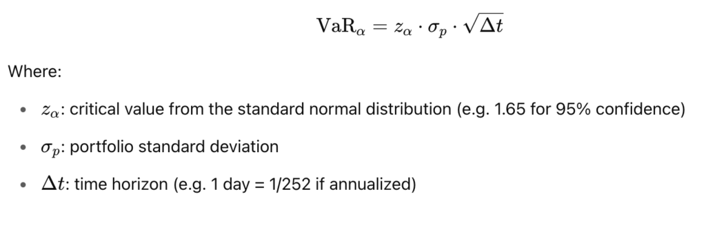
Value-at-Risk (VaR) estimates the potential loss in value of a portfolio over a given time period for a specified confidence level.

For a portfolio with normally distributed returns:

Let’s implement it:

#include <Eigen/Dense>
#include <iostream>
#include <cmath>

int main() {
    using namespace Eigen;

    // Portfolio weights
    Vector3d weights;
    weights << 0.5, 0.3, 0.2;

    // Covariance matrix of returns (annualized)
    Matrix3d cov;
    cov << 0.04, 0.006, 0.012,
           0.006, 0.09, 0.018,
           0.012, 0.018, 0.16;

    // Portfolio volatility (annualized)
    double variance = weights.transpose() * cov * weights;
    double sigma_p = std::sqrt(variance);

    // Convert to 1-day volatility
    double sigma_day = sigma_p / std::sqrt(252.0);

    // 95% confidence level
    double z_alpha = 1.65;
    double VaR = z_alpha * sigma_day;

    std::cout << "1-day 95% VaR: " << VaR << std::endl;

    return 0;
}

This code estimates the maximum expected portfolio loss over a single day with 95% confidence, assuming returns are normally distributed. The portfolio is composed of 3 assets with given weights and a known covariance matrix. We compute portfolio volatility using matrix operations, then scale it to daily terms and apply the standard normal quantile zαz_{\alpha}zα​.

Vector3d is equivalent to Eigen::Matrix<double, 3, 1>, representing a 3-dimensional column vector.

Matrix3d is equivalent to Eigen::Matrix<double, 3, 3>, representing a 3×3 matrix.

To run the code above, first install Eigen. I’m on Mac so:

brew install eigen

which installs the library in /usr/local/include/eigen3.

Then my CMakeLists.txt becomes:

cmake_minimum_required(VERSION 3.10)
project(eigenproject)

set(CMAKE_CXX_STANDARD 17)

include_directories(/usr/local/include/eigen3)

add_executable(var ../var.cpp)

which I use to compile:

mkdir build
cd build
cmake ..
make

And run:

➜  build ./var 
1-day 95% VaR: 0.0182592

This is a classic quant risk calculation that maps cleanly from equation to code with Eigen showing how linear algebra tools power real-world finance.

3. Boost: Statistical Foundations for Quant Models

Boost is a modular C++ library suite created in 1998 to provide high-quality, reusable code for systems programming and numerical computing. Many of its components, like smart pointers and lambdas, later shaped the C++ Standard Library. In quantitative finance, Boost is widely used for random number generation, probability distributions, statistical functions, and precise date/time manipulation. It’s not a finance-specific library, but a powerful foundation that supports core infrastructure in pricing engines and risk systems. For any quant working in C++, Boost is often running quietly behind the scenes. Boost is one of the most used and one of the best C++ libraries for quants.

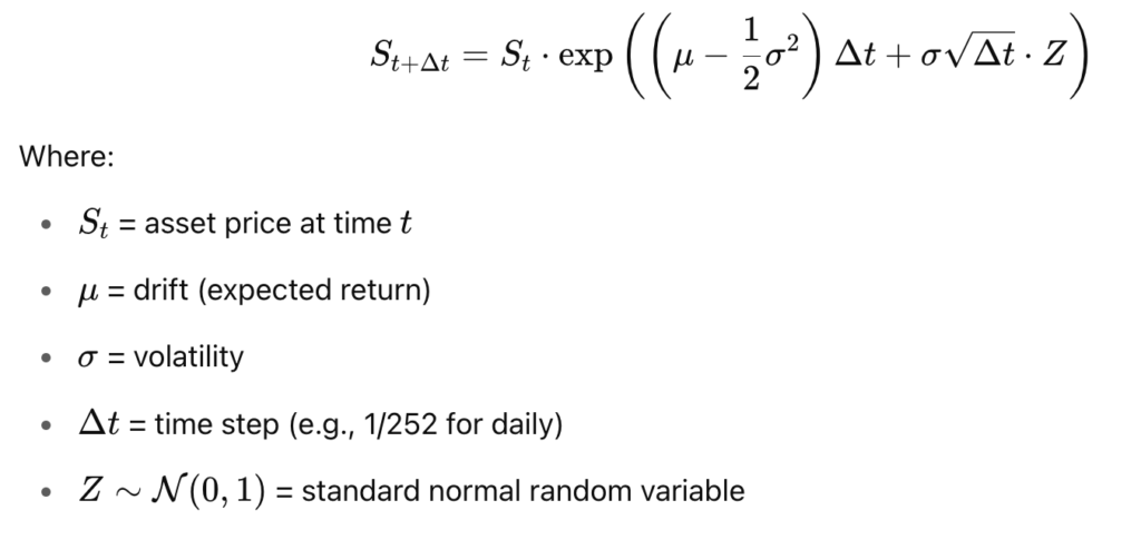
An example with Boost: simulate asset price path using Geometric Brownian Motion (GBM)

Geometric Brownian Motion (GBM) is the standard model for simulating asset prices in quantitative finance. It assumes that the asset price evolves continuously, driven by both deterministic drift (expected return) and stochastic volatility (random shocks).

This is the implementation using Boost:

#include <boost/random.hpp>
#include <iostream>
#include <vector>
#include <cmath>

int main() {
    const double S0 = 100.0;   // Initial price
    const double mu = 0.05;    // Annual drift
    const double sigma = 0.2;  // Annual volatility
    const double T = 1.0;      // 1 year
    const int steps = 252;     // Daily steps
    const double dt = T / steps;

    std::vector<double> path(steps + 1);
    path[0] = S0;

    // Random number generator (normal distribution)
    boost::mt19937 rng(42); // fixed seed
    boost::normal_distribution<> nd(0.0, 1.0);
    boost::variate_generator<boost::mt19937&, boost::normal_distribution<>> norm(rng, nd);

    for (int i = 1; i <= steps; ++i) {
        double Z = norm(); // sample from N(0, 1)
        path[i] = path[i - 1] * std::exp((mu - 0.5 * sigma * sigma) * dt + sigma * std::sqrt(dt) * Z);
    }

    for (double s : path)
        std::cout << s << "\n";

    return 0;
}

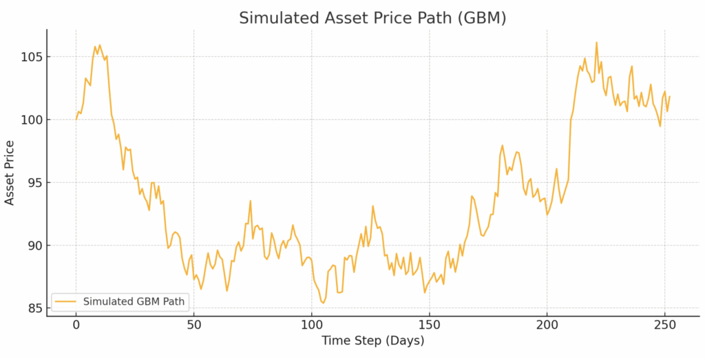
This simulation produces a single daily asset path over one year, which can be visualized, stored, or used to price derivatives via Monte Carlo methods.

How to run the code above?

First, as usual, we compile it with a basic CMakeLists.txt:

cmake_minimum_required(VERSION 3.10)
project(boostgmb)
set(CMAKE_CXX_STANDARD 17)
add_executable(gbm ../gbm.cpp)

Then:

mkdir build
cd build
cmake ..
make

Then run it to get the path:

➜  build ./gbm  
100
99.2103
98.1816
97.699
96.6464
95.4814
94.584
93.0535
94.5179
94.8266
95.1813
...

The Boost.Random library handles the normal distribution sampling cleanly and efficiently, an example of plot:

4. NLopt: Non Linear Calculus For Greeks

NLopt is a powerful, open-source library for non-linear optimization, created by Steven G. Johnson at MIT. One of the best C++ libraries for quants. It supports a wide range of algorithms, from local gradient-based methods to global optimizers like COBYLA and Nelder-Mead. In quant finance, NLopt shines in model calibration, curve fitting, and computing Greeks when closed-form derivatives aren’t available. It’s especially valuable when calibrating volatility surfaces, bootstrapping curves, or minimizing pricing model errors.

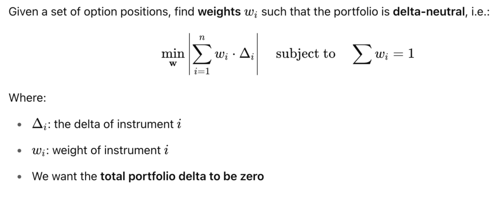
An example with NLopt: calibrate delta-neutral portfolio via optimization

Delta measures how much an option’s price changes with respect to small changes in the underlying asset’s price.
For example, a delta of 0.7 means the option gains $0.70 for every $1 move in the asset.
A delta-neutral portfolio is one where the net delta is zero, meaning small price moves in the underlying don’t affect the portfolio’s value.

This is a common hedging strategy used by quants and traders to reduce directional exposure.
The goal is to balance long and short positions to make the portfolio insensitive to short-term market movements.

Let’s implement it:

#include <nlopt.hpp>
#include <vector>
#include <iostream>
#include <cmath>

// Objective: minimize absolute portfolio delta
double objective(const std::vector<double>& w, std::vector<double>& grad, void* data) {
    std::vector<double>* deltas = static_cast<std::vector<double>*>(data);
    double total_delta = 0.0;

    for (size_t i = 0; i < w.size(); ++i)
        total_delta += w[i] * (*deltas)[i];

    return total_delta * total_delta;
}

// Constraint: weights must sum to 1
double weight_constraint(const std::vector<double>& w, std::vector<double>& grad, void*) {
    double sum = 0.0;
    for (double wi : w) sum += wi;
    return sum - 1.0;
}

int main() {
    std::vector<double> deltas = { 0.7, -0.4, 0.3 };
    int n = deltas.size();

    nlopt::opt opt(nlopt::LN_COBYLA, n);
    opt.set_min_objective(objective, &deltas);
    opt.add_equality_constraint(weight_constraint, nullptr, 1e-8);
    opt.set_xtol_rel(1e-6);

    std::vector<double> w(n, 1.0 / n); // initial guess
    double minf;
    nlopt::result result = opt.optimize(w, minf);

    std::cout << "Optimized weights for delta-neutral portfolio:\n";
    for (double wi : w) std::cout << wi << " ";
    std::cout << "\nPortfolio delta: " << minf << std::endl;

    return 0;
}

The function objective computes the portfolio delta using:

total_delta += w[i] * (*deltas)[i];

and returns its absolute value.

This is what NLopt tries to minimize to reach a delta-neutral state:

The function weight_constraint enforces the condition:

return sum - 1.0;

ensuring the sum of weights equals 1 (i.e. fully invested or net flat).

In main, we set up the optimizer with:

opt.set_min_objective(objective, &deltas);
opt.add_equality_constraint(weight_constraint, nullptr, 1e-8);

NLopt uses both the objective and the constraint during optimization.

An initial guess is given as equal weights:

std::vector<double> w(n, 1.0 / n);

Finally, we run the optimization:

opt.optimize(w, minf);

and print the optimized weights and final delta.

Now how to run this code?

First, I’ve installed nlopt:

brew install nlopt

And created a CMakeLists.txt linking the library:

cmake_minimum_required(VERSION 3.10)
project(deltaneutral)

set(CMAKE_CXX_STANDARD 17)

include_directories(/usr/local/include)
link_directories(/usr/local/lib)

add_executable(deltaneutral deltaneutral.cpp)

target_link_libraries(deltaneutral nlopt)

Now, I compile:

mkdir build
cd build
cmake ..
make

and run the executable:

➜  build ./deltaneutral 
Optimized weights for delta-neutral portfolio:
0.169295 0.525312 0.305393 
Portfolio delta: 1.409e-15

This structure shows how to balance a set of option positions to make the portfolio insensitive to small moves in the underlying — a core task in quant risk management.

I hope this article on the best C++ libraries for quants for informative, stay tuned for more!