C++ for Quants
  • Home
Author

Clement Daubrenet

Clement Daubrenet

Delta Greek Calculation
Greeks

Option Greeks in C++: Delta Calculation Explained

by Clement Daubrenet June 23, 2025

Delta is one of the most important Greeks in options pricing. It measures how sensitive an option’s price is to changes in the price of the underlying asset. How to perform a delta calculation? Let’s derive and it and calculate it in C++.

1. Derive the Delta Formula for a Call Option

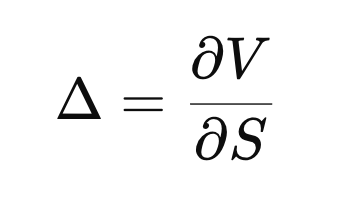
Delta is defined as the rate of change of an option’s price with respect to changes in the underlying asset price. In mathematical terms, it’s the first partial derivative of the option value V with respect to the underlying asset price S:

[math] \Large{\Delta = \frac{\partial V}{\partial S}} [/math]

Under the Black-Scholes framework, the price of a European call option is given by:

[math]\Large{C = S N(d_1) – K e^{-rT} N(d_2)}[/math]

Where:

  • S is the current spot price of the underlying
  • K is the strike price
  • r is the risk-free interest rate
  • T is the time to maturity
  • N(⋅) is the cumulative distribution function of the standard normal distribution
  • [math]d_1 = \frac{\ln(S/K) + \left(r + \frac{\sigma^2}{2} \right) T}{\sigma \sqrt{T}}[/math]
  • [math]d_2 = d_1 – \sigma \sqrt{T}[/math]

To compute the Delta of a call option, we differentiate the Black-Scholes formula with respect to S:

[math]\Large \frac{\partial C}{\partial S} = \frac{\partial}{\partial S} \left[ S N(d_1) – K e^{-rT} N(d_2) \right][/math]

Only the first term depends on S directly. The derivative of the first term requires the chain rule, since d1​ is a function of S as well. Thus:

[math]\Large \frac{\partial C}{\partial S} = N(d_1)[/math]

Therefore, the Delta of a European call option is:

[math]\Large \Delta_{\text{call}} = N(d_1)[/math]

2. Derive the Delta Formula For a Put Option

For a put option, we apply the same steps to the Black-Scholes formula for puts:

[math]\Large P = K e^{-rT} N(-d_2) – S N(-d_1)[/math]

Where:

  • S is the current spot price of the underlying
  • K is the strike price
  • r is the risk-free interest rate
  • T is the time to maturity
  • N(⋅) is the cumulative distribution function of the standard normal distribution
  • [math]d_1 = \frac{\ln(S/K) + \left(r + \frac{\sigma^2}{2} \right) T}{\sigma \sqrt{T}}[/math]
  • [math]d_2 = d_1 – \sigma \sqrt{T}[/math]

Differentiating:

[math]\Large \frac{\partial P}{\partial S} = -N(-d_1) = N(d_1) – 1[/math]

Hence, the Delta of a European put option is:

[math]\Large \Delta_{\text{put}} = N(d_1) – 1[/math]

3. Delta Calculation in C++ Without Library

We can simply implement the recipes above to calculate delta call and delta put:

#include <cmath>
#include <iostream>

// Cumulative normal distribution function
double norm_cdf(double x) {
    return 0.5 * std::erfc(-x / std::sqrt(2));
}

double black_scholes_delta(
    bool is_call,
    double S,     // Spot
    double K,     // Strike
    double T,     // Time to maturity
    double r,     // Risk-free rate
    double sigma  // Volatility
) {
    double d1 = (std::log(S / K) + (r + 0.5 * sigma * sigma) * T)
                / (sigma * std::sqrt(T));

    if (is_call) {
        return norm_cdf(d1);
    } else {
        return norm_cdf(d1) - 1.0;
    }
}


Then:

int main() {
    double S = 100.0;
    double K = 100.0;
    double T = 1.0;
    double r = 0.05;
    double sigma = 0.2;

    double delta_call = black_scholes_delta(true, S, K, T, r, sigma);
    double delta_put  = black_scholes_delta(false, S, K, T, r, sigma);

    std::cout << "Call Delta: " << delta_call << std::endl;
    std::cout << "Put Delta: "  << delta_put  << std::endl;
    return 0;
}

This is implements the analytical formula for Delta explicitly. It’s lightweight and very fast, great for educational or performance-critical code. It assumes flat rates and no dividends.

But what if you want something less generic?

4. Delta Calculation in C++ With Quantlib

Well, we can use the bazooka:

#include <ql/quantlib.hpp>
#include <iostream>

using namespace QuantLib;

int main() {
    Calendar calendar = TARGET();
    Date today(23, June, 2025);
    Settings::instance().evaluationDate() = today;

    // Common option parameters
    Real underlying = 100.0;
    Real strike = 100.0;
    Spread dividendYield = 0.0;
    Rate riskFreeRate = 0.05;
    Volatility volatility = 0.20;
    Date maturity = today + Period(1, Years);
    DayCounter dayCounter = Actual365Fixed();

    // Market data handles
    Handle<Quote> underlyingH(boost::shared_ptr<Quote>(new SimpleQuote(underlying)));
    Handle<YieldTermStructure> flatDividendTS(boost::shared_ptr<YieldTermStructure>(
        new FlatForward(today, dividendYield, dayCounter)));
    Handle<YieldTermStructure> flatRiskFreeTS(boost::shared_ptr<YieldTermStructure>(
        new FlatForward(today, riskFreeRate, dayCounter)));
    Handle<BlackVolTermStructure> flatVolTS(boost::shared_ptr<BlackVolTermStructure>(
        new BlackConstantVol(today, calendar, volatility, dayCounter)));

    boost::shared_ptr<BlackScholesMertonProcess> bsmProcess(
        new BlackScholesMertonProcess(underlyingH, flatDividendTS, flatRiskFreeTS, flatVolTS));

    // Loop over Call and Put options
    for (auto type : {Option::Call, Option::Put}) {
        std::string typeStr = (type == Option::Call ? "Call" : "Put");

        boost::shared_ptr<StrikedTypePayoff> payoff(new PlainVanillaPayoff(type, strike));
        boost::shared_ptr<Exercise> exercise(new EuropeanExercise(maturity));
        VanillaOption option(payoff, exercise);

        option.setPricingEngine(boost::shared_ptr<PricingEngine>(
            new AnalyticEuropeanEngine(bsmProcess)));

        std::cout << typeStr << " Delta: " << option.delta() << std::endl;
    }

    return 0;
}

✅ The QuantLib implementation:

  • Wraps the same math, but within a complete pricing engine (AnalyticEuropeanEngine).
  • Uses market objects like Quote, YieldTermStructure, and BlackVolTermStructure, which can evolve over time.
  • Supports dividends, yield curves, non-constant volatility, and more.

In a word, it’s heavier but more flexible and extensible, making it better suited for production systems or derivatives desks.

5. Let’s Run Both and Compare?

Let’s start with the first version, after compiling and running:

➜  ./delta_vanilla                                                              
Call Delta: 0.636831
Put Delta: -0.363169

Now, the Quantlib version:

➜  build ./delta_quantlib 
Call Delta: 0.636831
Put Delta: -0.363169

The exact same!

What about execution time?

For the first version, it’s instant, <<0.01s:

➜  build time ./delta_vanilla 

./delta_vanilla  0.00s user 0.00s

For the Quantlib version, ~0.01s, slightly slower:

➜  build time ./delta_quantlib

./delta_quantlib  0.00s user 0.01s

4. Summarize Both Implementations for Delta Calculation

FeatureVanillaQuantLib
Analytical Delta✅ Yes✅ Yes
Dividend support❌ No✅ Yes
Yield curve support❌ No✅ Yes
Vol surface support❌ No✅ Yes
Performance⚡ Very fast🐢 Slower (but flexible)
Good for learning✅ Absolutely✅ But more complex
Good for real-world desks❌ Not sufficient✅ Industry standard

If you’re writing an educational article or prototyping, the vanilla version is perfect. If you’re integrating with a full market data and pricing system, QuantLib is the go-to.

June 23, 2025 0 comments
C++ quant jobs
Jobs

C++ Quantitative Developers: A Skyrocketing Job Market

by Clement Daubrenet June 23, 2025

The job market for C++ quantitative developers is experiencing a major surge. Driven by the relentless demand for low-latency execution, many hedge funds and trading firms are ramping up hiring. C++ remains the gold standard for performance-critical systems in finance — and its dominance is growing.
Top firms like Citadel, Jane Street, and Jump Trading are offering eye-watering compensation packages to attract talent.

In London, New York, and Singapore, six-figure base salaries are now entry-level — with total comp often exceeding $500k.
Real-time risk, high-frequency trading, and exotic derivatives desks all need C++ expertise.
The rise of data-driven modeling has only reinforced the need for tight integration between quant models and execution engines.
Firms want devs who can code, optimize, and understand the math — and C++ sits at that intersection.
With competition heating up, even junior roles now demand systems-level thinking and modern C++ fluency.
For quants and devs alike, now is a golden moment to ride the C++ finance wave.

1. Some Data about Salaries

The demand for C++ Quant Developers in the UK has exploded — and salaries reflect it. The median salary has jumped to £170,000, up 17.24% year-on-year, continuing a multi-year upward trend. Even more striking, the 10th percentile salary has more than doubled since 2024, rising from £56,250 to £135,000, suggesting that entry-level roles are commanding mid-career paychecks.

The number of permanent roles has also nearly doubled in a year, with 33 positions advertised versus just 18 the year prior. C++ quant roles now represent 0.058% of all UK job ads, a 3.6x increase in relative share — highlighting how niche, high-impact, and in-demand this skillset has become.

Whether you’re a seasoned systems programmer or a mathematically-minded developer eyeing the finance sector, the numbers don’t lie: it’s a C++ quant boom.

2. The Trend is Volatile but Clearly Goes Up

This 20-year salary trend graph shows a clear and accelerating rise in compensation for C++ Quantitative Developers in the UK. After a decade of relative stability from 2005 to 2015, salaries began a marked upward shift around 2018, aligning with the growing demand for low-latency systems and tighter model-to-execution integration. Since 2020, volatility has increased — but so has the upside. The median salary line (orange) now sits firmly above £150,000, with the top 10% breaching the £200,000+ mark. Even the 25th percentile has climbed significantly, pointing to strong tailwinds across all seniority levels. As of mid-2025, the trend is steeply upward — a reflection of how C++ has reasserted itself as a core technology in quant finance.

3. The Tools, Skills, Exposure and Libraries Required

The C++ Quant Developer role is no longer just about knowing C++. According to data from the six months leading up to June 2025, Low Latency (93.94%), Equities, and Hedge Funds appear alongside C++ in nearly all job ads, signaling a strong demand for developers who understand real-time execution environments in capital markets.

Interestingly, Python (90.91%) appears just as frequently — reinforcing the industry’s shift toward hybrid devs who can optimize in C++ and prototype in Python.
Skills like Linux, Multithreading, Algorithms, and Data Structures remain core, while mentions of Boost, Test Automation, and Order Management show that system reliability and front-office tooling are just as valued as raw performance.

Whether it’s Quantitative Trading, Market Making, or Greenfield Projects, this skill map clearly shows that modern quant devs must span systems engineering, financial markets, and rapid prototyping — a rare and highly-paid blend.

4. Conclusion

The data is unambiguous: C++ Quantitative Developers are among the most sought-after professionals in finance today. Salaries are surging, with median comp hitting £170,000, and top roles exceeding £200,000+. Even the lowest percentiles are rising fast — entry-level is no longer “junior” in pay. Demand has more than doubled year-on-year, with job postings climbing steadily. C++ sits at the core of high-frequency trading, real-time risk, and complex derivatives pricing.

But employers aren’t just hiring C++ coders — they want versatile technologists. Fluency in Python, Linux, Multithreading, and Low Latency architecture is essential. Firms want devs who can design systems, optimize them, and understand market dynamics. This is no longer a back-office role — the Front Office is calling, and it pays.

Whether you’re a quant with systems chops or a dev learning finance, now is the time to strike. The most competitive candidates understand both algorithms and alpha. They build fast, test fast, and deploy into production with confidence. The C++ quant role is evolving — it’s becoming broader, better-paid, and more central to business.

This is not a bubble. It’s a structural shift. As market infrastructure becomes more automated and data-hungry, firms will invest heavily in top-tier engineering. That means a long runway for anyone investing in the right skills now.
If you’ve been on the fence about switching into finance — consider this your signal. And if you’re already here: it’s time to double down on your edge.

June 23, 2025 0 comments
tree shap model
Credit Risk

Attribution Modeling for Credit PnL Using TreeSHAP

by Clement Daubrenet June 23, 2025

In modern credit trading, understanding why PnL moves is just as important as tracking that it moved.
When billions of data points flow through trading systems daily, intuition and heuristics fall short.
This article presents a scalable method for attributing PnL changes to specific credit risk drivers.
We model feature deltas — changes in exposure, spreads, and counterparty metrics — across time.


We train a LightGBM model to learn nonlinear relationships between deltas and ΔPnL.
Then, we apply TreeSHAP to extract the top features responsible for each credit-related PnL movement.
The result is a transparent, auditable, per-entity view of what caused the last PnL move.
This is not prediction, it’s attribution — a diagnostic engine for credit risk.

1. Introduction: The Need for Attribution, Not Prediction

Credit-related PnL refers to profit and loss driven by credit risk exposure — such as changes in counterparty credit spreads, rating downgrades, or shifts in default probabilities.
It captures the financial impact of events like widening CDS, growing exposures, or collateral changes, rather than market or operational effects.


For traders, a sudden loss tied to a counterparty matters less than knowing which risk factor caused it.
For quants, understanding nonlinear relationships between inputs and PnL is key to model trust and validation.
And for risk teams, attribution supports regulatory reporting, stress testing, and early warnings.
But with data at the scale of billions of deltas, traditional methods fail to offer clear answers.
We propose a hybrid pipeline: use Python to train a LightGBM model on feature deltas and PnL deltas.
Then apply TreeSHAP to explain which deltas caused most of the PnL movement.
For real-time inference, we port the model and SHAP logic to a high-performance C++ backend.
The result: an explainable, scalable, and production-ready system for credit PnL attribution at scale.

2. Data Design: Tracking the Right Deltas

Every 15 minutes, a new snapshot arrives — a high-dimensional vector (10,000+ features) representing the full state of the trading system: exposure, spreads, counterparty credit ratings, margin calls, instrument properties, and more.

This raw data isn’t yet meaningful. To extract signal, we compute deltas: changes in features between consecutive time windows. These represent what moved.

Alongside the feature deltas, we compute the PnL delta, giving us a supervised signal to explain: what caused the profit or loss change since the last window?

We filter and engineer meaningful features — credit spreads, counterparty ratings, net exposure, sector-level aggregates — to reduce noise and emphasize credit drivers.

Using deltas instead of raw levels is key. Most credit features are auto-correlated or slow-moving — a high exposure value tells us less than a sudden increase in exposure.

The delta of a credit spread or notional tells us more about risk events, decisions, or systemic shifts than the absolute value alone.

By modeling dPnL ~ Δ_features, we move from static snapshots to causal attribution.

📄 Mocked Extract of Delta Dataset

timestampentityΔ_exposureΔ_cds_bnpΔ_rating_scoreΔ_sector_riskΔPnL
2025-06-23 10:00:00trader_01+2.3M+0.018-1+0.07-4.21M
2025-06-23 10:15:00trader_01-1.1M-0.0050-0.03+2.73M
2025-06-23 10:30:00trader_01+0.4M+0.00200-1.00M
  • Δ_exposure: Notional delta to counterparties
  • Δ_cds_bnp: Change in BNP CDS (in decimal)
  • Δ_rating_score: Discrete rating movement (e.g., 1 = downgrade)
  • Δ_sector_risk: Change in weighted average sector risk score
  • dPnL: Total change in credit-related PnL

We will drastically increase the dimensionality of those with 10k columns and 1 million rows.

We generate millions of entries in “delta_features.csv” and millions of delta PnLs in “delta_pnl.csv”

3. Modeling: Training a Gradient Boosted Tree on Deltas

To prepare for TreeSHAP attribution in this credit delta → PnL delta setup, you’ll want to use a LightGBM regression model that emphasizes explainability, stability, and performance.

✅ Goal:

  • Train a LightGBM model (Δfeatures → ΔPnL)
  • Export the model (model.txt)
  • Optionally export samples for testing C++ inference

🧠 File: train_model.py


import lightgbm as lgb
import pandas as pd

# Load delta feature and delta PnL data
X = pd.read_csv("delta_features.csv")
y = pd.read_csv("delta_pnl.csv")

# Train model
params = {
    "objective": "regression",
    "metric": "rmse",
    "learning_rate": 0.03,
    "num_leaves": 64,
    "feature_fraction": 0.6,
    "bagging_fraction": 0.8,
    "bagging_freq": 5,
    "lambda_l1": 0.1,
    "lambda_l2": 1.0,
    "min_data_in_leaf": 50,
    "verbose": -1
}
model = lgb.train(lgb.Dataset(X, label=y), params, num_boost_round=200)

# Save model
model.save_model("model.txt")

# Export a row (e.g., for test inference)
row_index = 12345
X.iloc[[row_index]].to_csv("sample_row.csv", index=False)
y.iloc[[row_index]].to_csv("sample_label.csv", index=False)

Then we can run the inferrence:

import pandas as pd
import shap
import lightgbm as lgb

# Load model and data
model = lgb.Booster(model_file="model.txt")          # Trained LGBM model
X = pd.read_csv("sample_row.csv")         # Latest 15-min features (deltas)
y_pnl = pd.read_csv("sample_label.csv")          # Actual PnL deltas (optional)

# Run SHAP
explainer = shap.TreeExplainer(model)
shap_values = explainer.shap_values(X)

# For a specific row (e.g. last 15-min observation)
row = 0
shap_row = shap_values[row]

# Create attribution table
explained = pd.DataFrame({
    "feature": X.columns,
    "shap_value": shap_row,
    "feature_value": X.iloc[row]
}).sort_values(by="shap_value", key=abs, ascending=False)

# Add cumulative contribution
explained["cum_impact"] = explained["shap_value"].cumsum()
total_impact = abs(explained["shap_value"]).sum()
explained["cum_percent"] = abs(explained["shap_value"]).cumsum() / total_impact

# Output: top features responsible for 90% of the PnL move
top_contributors = explained[explained["cum_percent"] <= 0.9]
print(top_contributors)

4. Results

📦 Output Example

      feature      shap_value  feature_value  cum_impact  cum_percent
23 spread_delta 0.68 12.0 0.68 0.42
14 curve_1y 0.51 3.2 1.19 0.72
9 exposure_bond 0.33 54.1 1.52 0.92

This shows:

  • The features most responsible for the ΔPnL for that 15-min slice
  • Their raw SHAP impact
  • How much of the total impact they cumulatively explain

June 23, 2025 0 comments
Implied Volatility
Volatility

Compute the Implied Volatility for a Call Option in C++

by Clement Daubrenet June 21, 2025

Volatility is a cornerstone concept in finance, used to measure the degree of variation in the price of a financial instrument. Two of the most commonly referenced types are Implied Volatility (IV) and Historical Volatility (HV), and while they both aim to assess risk, they do so from different perspectives.

Implied Volatility is forward-looking. Derived from option prices using models like Black-Scholes, it reflects the market’s expectations of future price movement. Higher IV typically signals greater anticipated risk or uncertainty.

HV is objective and purely data-driven, while IV incorporates market sentiment and supply-demand dynamics in the options market.

1. Derive Black-Scholes PDE Solution for European Call Options

To derive implied volatility from the Black-Scholes model, you’re essentially trying to find the volatility (σ) that, when plugged into the Black-Scholes formula, yields the market price of the option.

Let’s start from Black-Scholes.

[math]
\Large{dS_t = \mu S_t \, dt + \sigma S_t \, dW_t}
[/math]

is a stochastic differential equation (SDE) — it’s the core model behind how asset prices evolve over time in the Black-Scholes framework.


🔍 Term-by-Term Breakdown

SymbolMeaning
[math] S_t​ [/math]The price of the asset (e.g., stock) at time ttt
[math] dS_t [/math]The infinitesimal change in the asset price over a small time interval
[math] \mu [/math] The drift — average rate of return (expected % growth per unit time)
dtA very small time interval (infinitesimal)
[math] \sigma [/math]The volatility — standard deviation of returns per unit time (how “noisy” the price is)
[math] dWt [/math]A random shock, also called a Wiener process or Brownian motion increment. Represents randomness.

The formula models price changes as having two components:

A deterministic part:

[math] \Large{\mu S_t \, dt} [/math]

This is the trend — the predictable, average growth over time.

A stochastic part:

[math] \Large{\sigma S_t \, dW_t} [/math]

This is the randomness — the noise or uncertainty in price movements.

  • [math] \sigma [/math] scales the size of the randomness.
  • [math] dW_t​ [/math] brings in randomness from a standard Brownian motion: the mean is 0 and the variance is dt

A first thing to do to reach the implied volatility question is to notice that to price options, we don’t use [math] mu [/math] because investors care about risk-adjusted returns.

Instead, we use r for the risk-neutral measure [math] \mathbb{Q} [/math], where:

[math] \Large{dS_t = r S_t \, dt + \sigma S_t \, dW_t^{\mathbb{Q}}} [/math]

  • The drift becomes r, the risk-free rate.
  • The randomness remains via [math] \sigma [/math] and [math] dW_t [/math]

🔍 Let’s define the call option price


[math]\Large{ C(t,S_t​)=price of a call option} [/math]

After a bit of work that we will not do in this article, we can derive the Black-Scholes PDE:

[math] \Large{\frac{\partial C}{\partial t} + r S_t \frac{\partial C}{\partial S} + \frac{1}{2} \sigma^2 S_t^2 \frac{\partial^2 C}{\partial S^2} – r C = 0} [/math]

Solving this PDE with the terminal condition:

[math] \Large{C(T, S_T) = \max(S_T – K, 0)} [/math]

gives us the option price at time t=0:

[math] \Large{C(\sigma) = S_0 \Phi(d_1) – K e^{-rT} \Phi(d_2)} [/math]

where:

[math] \Large{d_1 = \frac{\ln(S_0 / K) + (r + \frac{1}{2} \sigma^2) T}{\sigma \sqrt{T}}} [/math]

And

[math] \Large{d_2 = d_1 – \sigma \sqrt{T}} [/math]

2. Determine the Equation to Solve to get the Implied Volatility

We now take the market-observed option price [math] C_{market} [/math] and ask:

“What value of [math] \sigma [/math] makes the Black-Scholes price equal the market price?”

So we define the equation to solve:

[math] \Large{f(\sigma) = C(\sigma) \, – C_{\text{market}} = 0} [/math]

Since C(σ)C(\sigma)C(σ) involves Φ(d1)\Phi(d_1)Φ(d1​) and d1d_1d1​ contains σ\sigmaσ both in the numerator and denominator, there is no closed-form algebraic solution.

We solve it using numerical methods:

  • Brent’s method (robust)
  • Newton-Raphson (faster, requires Vega)
  • Bisection (simple, slower)

What does it mean to solve that equation in a real-world context?

🧮 Example

Let’s say the following is true today:

ParameterValue
[math] S_0 [/math]​ (stock price)$100
K (strike)$105
T (time to maturity)30 days ≈ 0.0822 years
r (risk-free rate)5% = 0.05
[math] C_{market} [/math] option price from market$2.50

👇 Now We Need To Solve:

[math] \Large{f(\sigma) = C(\sigma) – 2.50 = 0} [/math]

You plug different values of [math] \sigma [/math] into the Black-Scholes formula:

[math] \Large{C(\sigma) = S_0 \Phi(d_1) – K e^{-rT} \Phi(d_2)} [/math]

where:

[math] \Large{d_1 = \frac{\ln(S_0 / K) + (r + \frac{1}{2} \sigma^2) T}{\sigma \sqrt{T}}} [/math]

[math] \Large{d_2 = d_1 – \sigma \sqrt{T}} [/math]

And iterate until:

[math] \Large{C(\sigma) \approx 2.50} [/math].

So, how do we iterate to solve the volatility equation?

3. Use Quantlib to Solve the Implied Volatility Equation

Quantlib will solve that equation with a numerical method.

Here is the code for the example above:

#include <ql/quantlib.hpp>
#include <iostream>

using namespace QuantLib;

int main() {
    Calendar calendar = TARGET();
    Date today = Date::todaysDate();
    Settings::instance().evaluationDate() = today;

    // Option parameters
    Option::Type optionType = Option::Call;
    Real underlying = 100.0;
    Real strike = 105.0;
    Rate riskFreeRate = 0.05;
    Volatility initialVol = 0.20; // Just an initial guess
    Date maturity = calendar.advance(today, Period(30, Days));  // 30-day maturity
    Real marketPrice = 2.50;

    DayCounter dayCounter = Actual365Fixed();
    Handle<Quote> underlyingH(boost::shared_ptr<Quote>(new SimpleQuote(underlying)));

    // Constructing the yield curve and flat volatility surface
    Handle<YieldTermStructure> flatTermStructure(
        boost::shared_ptr<YieldTermStructure>(
            new FlatForward(today, riskFreeRate, dayCounter)));

    Handle<BlackVolTermStructure> flatVolTS(
        boost::shared_ptr<BlackVolTermStructure>(
            new BlackConstantVol(today, calendar, initialVol, dayCounter)));

    boost::shared_ptr<StrikedTypePayoff> payoff(
        new PlainVanillaPayoff(optionType, strike));

    boost::shared_ptr<Exercise> exercise(
        new EuropeanExercise(maturity));

    EuropeanOption option(payoff, exercise);

    Handle<YieldTermStructure> flatDividendTS(
    boost::shared_ptr<YieldTermStructure>(
        new FlatForward(today, 0.0, dayCounter)));

    boost::shared_ptr<BlackScholesMertonProcess> bsmProcess(
        new BlackScholesMertonProcess(underlyingH, 
                                      flatDividendTS, 
                                      flatTermStructure, 
                                      flatVolTS));

    // Calculate implied volatility
    try {
        Volatility impliedVol = option.impliedVolatility(
            marketPrice, bsmProcess, 1e-6, 100, 0.0001, 4.0);
        std::cout << "Implied Volatility: " << impliedVol << std::endl;
    } catch (std::exception& e) {
        std::cerr << "Error calculating implied volatility: " << e.what() << std::endl;
    }

    return 0;
}

after:

brew install quantlib

and setting up your CMakeLists.txt:

cmake_minimum_required(VERSION 3.10)
project(QuantLibImpliedVolExample)

set(CMAKE_CXX_STANDARD 17)

find_package(PkgConfig REQUIRED)
pkg_check_modules(QUANTLIB REQUIRED QuantLib)

include_directories(${QUANTLIB_INCLUDE_DIRS})
link_directories(${QUANTLIB_LIBRARY_DIRS})

add_executable(implied_vol src/volatility.cpp)
target_link_libraries(implied_vol ${QUANTLIB_LIBRARIES})

and now you can compile:

mkdir build
cd build
cmake ..
make

Eventually, you can run the executable:

> ./implied_vol
Implied Volatility: 0.318886
June 21, 2025 0 comments
Options Pricing Quantlib
Libraries

Develop a European Style Option Pricer with Quantlib

by Clement Daubrenet June 20, 2025

In this tutorial, we’ll walk through how to build a European style option pricer for the S&P 500 (SPX) using C++ and the QuantLib library. Although SPX tracks an American index, its standard listed options are European-style and cash-settled, making them ideal for analytical pricing models like Black-Scholes.

We’ll use historical market data to simulate a real-world scenario, define the option contract, and compute its price using QuantLib’s powerful pricing engine. Then, we’ll visualize how the option’s value changes in response to different parameters — such as volatility, strike price, time to maturity, and the risk-free rate.

1. What’s a European Style Option?

A call option is a financial contract that gives the buyer the right (but not the obligation) to buy an underlying asset at a fixed strike price on or before a specified expiration date.

The buyer pays a premium for this right. If the asset’s market price rises above the strike price, the option becomes profitable, as it allows the buyer to acquire the asset (or cash payout, in the case of SPX) for less than its current value.

In the case of SPX options, which are European-style and cash-settled, the option can only be exercised at expiration, and the buyer receives the difference in cash between the spot price and the strike price — if the option ends up in the money.

✅ Profit Scenario — Call Option Buyer

A trader buys a call option with the following terms:

ParameterValue
Strike price$105
Premium paid$5
Expiration dateSeptember 20, 2026
Break-even price$110

This call option gives the trader the right (but not the obligation) to buy the underlying stock for $105 on September 20, 2026, no matter how high the stock price goes.

📊 Profit and Loss Outcomes:

–If the stock is below $105 on expiry:
The option expires worthless.
The maximum loss is the premium paid, which is $5.

–If the stock is exactly $110 at expiry:
The option is in the money, but just enough to break even:
(110−105)−5=0

–If the stock is above $110:
The trader earns unlimited upside beyond the break-even price.

2. The Case of a SPX Call Option

Let’s now consider a realistic scenario involving an SPX call option — a European-style, cash-settled derivative contract on the S&P 500 index.

Suppose a trader considers a call option on SPX with the following characteristics:

ParameterValue
Strike price4200
Premium paid$50
Expiration dateSeptember 20, 2026
Break-even price4250

This contract gives the buyer the right to receive a cash payout equal to the difference between the SPX index value and the strike price, if the index finishes above 4200 at expiry. Because SPX options are European-style, the option can only be exercised at expiration, and the payout is settled in cash.

This option can be named with different conventions:

Depending on the context (exchange, data provider, or trading platform), the same SPX option can be referred to using various naming conventions. Here are the most common formats:

Format TypeExampleDescription
Human-readableSPX-4200C-2026-09-20Readable format: underlying, strike, call/put, expiration date
OCC Standard FormatSPX260920C04200000Used by the Options Clearing Corporation: YYMMDD + C/P + 8-digit strike
Bloomberg-styleSPX US 09/20/26 C4200 IndexUsed in terminals like Bloomberg
Yahoo Finance-styleSPX Sep 20 2026 4200 CallOften seen on retail platforms and data aggregators

All of these refer to the same contract: a European-style SPX call option with a strike price of 4200, expiring on September 20, 2026.

3. Develop a SPX US 09/20/26 C4200 European Style Option Pricer

This C++ example uses QuantLib to price a European-style SPX call option by first calculating its implied volatility from a given market price, then re-pricing the option using that implied vol.

It’s a simple, clean way to bridge real-world option data with model-based pricing.
Perfect for understanding how traders extract market expectations from prices.

#include <ql/quantlib.hpp>
#include <iostream>

using namespace QuantLib;

int main() {
    // Set today's date
    Date today(20, June, 2026);
    Settings::instance().evaluationDate() = today;

    // Option parameters
    Real strike = 4200.0;
    Date expiry(20, September, 2026);
    Real marketPrice = 150.0;   // Market price of the call
    Real spot = 4350.0;         // SPX index level
    Rate r = 0.035;             // Risk-free rate
    Volatility volGuess = 0.20; // Initial guess

    // Day count convention
    DayCounter dc = Actual365Fixed();

    // Set up handles
    Handle<Quote> spotH(boost::make_shared<SimpleQuote>(spot));
    Handle<YieldTermStructure> rH(boost::make_shared<FlatForward>(today, r, dc));
    Handle<BlackVolTermStructure> volH(boost::make_shared<BlackConstantVol>(today, TARGET(), volGuess, dc));

    // Build option
    auto payoff = boost::make_shared<PlainVanillaPayoff>(Option::Call, strike);
    auto exercise = boost::make_shared<EuropeanExercise>(expiry);
    EuropeanOption option(payoff, exercise);

    auto process = boost::make_shared<BlackScholesProcess>(spotH, rH, volH);

    // Calculate implied volatility
    Volatility impliedVol = option.impliedVolatility(marketPrice, process);
    std::cout << "Implied Volatility: " << impliedVol * 100 << "%" << std::endl;

    // Re-price using implied vol
    Handle<BlackVolTermStructure> volH_real(boost::make_shared<BlackConstantVol>(today, TARGET(), impliedVol, dc));
    auto process_real = boost::make_shared<BlackScholesProcess>(spotH, rH, volH_real);
    option.setPricingEngine(boost::make_shared<AnalyticEuropeanEngine>(process_real));

    std::cout << "Recalculated Option Price: " << option.NPV() << std::endl;
    return 0;
}

🔍 Explanation of the Steps

  1. Set market inputs: We define the option’s parameters, spot price, risk-free rate, and the option’s market price.
  2. Estimate implied volatility: QuantLib inverts the Black-Scholes formula to solve for the volatility that matches the market price.
  3. Reprice with implied vol: We plug the implied volatility back into the model to confirm the match and prepare for any further analysis (Greeks, charts, etc.).

4. Ideas of Experiments

Once your European style option pricer works for this SPX call option, you can extend it with experiments to better understand option dynamics and sensitivities:

  1. Vary the Spot Price
    Observe how the option value changes as SPX moves from 4000 to 4600. Plot a payoff curve at expiry and at time-to-expiry.
  2. Strike Sweep (Volatility Smile)
    Keep the expiry fixed and compute implied volatility across a range of strike prices (e.g., 3800 to 4600). Plot the resulting smile or skew.
  3. Volatility Sensitivity (Vega Analysis)
    Change implied volatility from 10% to 50% and plot the change in option price. This shows how much the price depends on volatility.
  4. Time to Expiry (Theta Decay)
    Fix all inputs and reduce the time to maturity in steps (e.g., 90 → 60 → 30 → 1 day). Plot how the option price decays over time.
  5. Compare Historical vs Implied Vol
    Calculate historical volatility from past SPX prices and compare it to the implied vol from market pricing. Plot both for the same strike/expiry.
  6. Greeks Across Time or Price
    Plot delta, gamma, vega as functions of SPX price or time to expiry using QuantLib’s option.delta() etc.
  7. Stress Test Scenarios
    Combine spot drops and volatility spikes to simulate market panic — useful to understand hedging behavior.

Each of these can generate powerful charts or tables to enhance your article or future dashboards. Let me know if you’d like example plots or code snippets for any of them.

June 20, 2025 0 comments
C++ libs for quants
Libraries

Best C++ Libraries for Quants: An Overview

by Clement Daubrenet June 19, 2025

C++ is widely used in quant finance for its speed and control. To build pricing engines, risk models, and simulations efficiently, quants rely on specific libraries. This article gives a quick overview of the most useful ones:

  • QuantLib – derivatives pricing and fixed income
  • Eigen – fast linear algebra
  • Boost – utilities, math, random numbers
  • NLopt – non-linear optimization

Each library is explained with use cases and code snippets: let’s discover the best C++ libraries for quants.

1. Quantlib: The Ultimate Quant Toolbox

QuantLib is an open-source C++ library for modeling, pricing, and managing financial instruments.
It was started in 2000 by Ferdinando Ametrano and later developed extensively by Luigi Ballabio, who remains one of its lead maintainers.

QuantLib is used by several major institutions and fintech firms. J.P. Morgan and Bank of America have referenced it in quant research roles and academic work. Bloomberg employs developers who have contributed to the library. OpenGamma, StatPro, and TriOptima have built tools on top of it. ING has published QuantLib-based projects on GitHub. It’s also used in academic settings like Oxford, ETH Zurich, and NYU for teaching quantitative finance. While not always publicly disclosed, QuantLib remains a quiet industry standard across banks, hedge funds, and research labs.

An example with Quantlib: Black-Scholes European call option pricing

This example calculates the fair price of a European call option using the Black-Scholes model. It sets up the option parameters, market conditions, and uses QuantLib’s analytic engine to compute the net present value (NPV) of the option.

The Black-Scholes-Merton model provides a closed-form solution for the price of a European call option (which can only be exercised at maturity).

A call option is a financial contract that gives the buyer the right, but not the obligation, to buy an underlying asset (like a stock) at a specified strike price (K) on or before a specified maturity date (T).
The buyer pays a premium for this right. If the asset price STS_TST​ at maturity is higher than the strike price, the call is “in the money” and can be exercised for profit.

Let’s implement it with Quantlib:

#include <ql/quantlib.hpp>
#include <iostream>

int main() {
    using namespace QuantLib;

    Calendar calendar = TARGET();
    Date settlementDate(19, June, 2025);
    Settings::instance().evaluationDate() = settlementDate;

    // Option parameters
    Option::Type type(Option::Call);
    Real underlying = 100;
    Real strike = 100;
    Spread dividendYield = 0.00;
    Rate riskFreeRate = 0.05;
    Volatility volatility = 0.20;
    Date maturity(19, December, 2025);
    DayCounter dayCounter = Actual365Fixed();

    // Construct the option
    ext::shared_ptr<Exercise> europeanExercise(new EuropeanExercise(maturity));
    Handle<Quote> underlyingH(ext::make_shared<SimpleQuote>(underlying));
    Handle<YieldTermStructure> flatTermStructure(
        ext::make_shared<FlatForward>(settlementDate, riskFreeRate, dayCounter));
    Handle<YieldTermStructure> flatDividendTS(
        ext::make_shared<FlatForward>(settlementDate, dividendYield, dayCounter));
    Handle<BlackVolTermStructure> flatVolTS(
        ext::make_shared<BlackConstantVol>(settlementDate, calendar, volatility, dayCounter));

    ext::shared_ptr<StrikedTypePayoff> payoff(new PlainVanillaPayoff(type, strike));
    ext::shared_ptr<BlackScholesMertonProcess> bsmProcess(
        new BlackScholesMertonProcess(underlyingH, flatDividendTS, flatTermStructure, flatVolTS));

    EuropeanOption europeanOption(payoff, europeanExercise);
    europeanOption.setPricingEngine(ext::make_shared<AnalyticEuropeanEngine>(bsmProcess));

    std::cout << "Option price: " << europeanOption.NPV() << std::endl;

    return 0;
}

Here’s how the key financial parameters map into the QuantLib code:

Option::Type type(Option::Call);  // We are pricing a European CALL
Real underlying = 100;            // Current asset price S₀ = 100
Real strike = 100;                // Strike price K = 100
Spread dividendYield = 0.00;      // Assumes zero dividend payments
Rate riskFreeRate = 0.05;         // Constant risk-free rate r = 5%
Volatility volatility = 0.20;     // Annualized volatility σ = 20%
Date maturity(19, December, 2025); // Option maturity (T ~ 0.5 years if priced in June 2025)

Supporting Structures

  • EuropeanExercise — specifies the option is European-style (only exercised at maturity).
  • PlainVanillaPayoff — defines the payoff max⁡(ST−K,0)\max(S_T – K, 0)max(ST​−K,0).
  • FlatForward and BlackConstantVol — assume constant risk-free rate and volatility.
  • BlackScholesMertonProcess — encapsulates the stochastic process assumed by the model.

Pricing Engine

Eventually, this line tells QuantLib to use the closed-form Black-Scholes solution for pricing the option.

europeanOption.setPricingEngine(
    ext::make_shared<AnalyticEuropeanEngine>(bsmProcess));

and, in the end of the code, we execute:

std::cout << "Option price: " << europeanOption.NPV() << std::endl;

.NPV() in QuantLib stands for Net Present Value.

In the context of an option or any financial instrument, NPV() returns the theoretical fair price of the instrument as calculated by the chosen pricing engine (in this case, the Black-Scholes analytic engine for a European call).

Now how to run it? First, install Quantlib. If you’re on Mac, it’s as simple as:

brew install quantlib

Now let’s compile it by adding a CMakeLists.txt:

cmake_minimum_required(VERSION 3.10)
project(QuantLibTestExample)

set(CMAKE_CXX_STANDARD 17)

find_package(PkgConfig REQUIRED)
pkg_check_modules(QUANTLIB REQUIRED QuantLib)

include_directories(${QUANTLIB_INCLUDE_DIRS})
link_directories(${QUANTLIB_LIBRARY_DIRS})

add_executable(pricer ../pricer.cpp)
target_link_libraries(pricer ${QUANTLIB_LIBRARIES})

Let’s create a build directory and run cmake:

mkdir build
cd build
cmake ..
make

And run the pricer:

➜  build ./pricer        
Option price: 6.89984

It was easy, right? Yes, Quantlib is probably among the best C++ libraries for quants. If not the best.

2. Eigen: The Quant’s Matrix Powerhouse

Eigen is a C++ template library for linear algebra, created by Benoît Jacob and first released in 2006.

Designed for speed, accuracy, and ease of use, it quickly became a favorite in scientific computing, robotics, and machine learning — and naturally found its place in quantitative finance. Eigen is header-only, highly optimized, and supports dense and sparse matrix operations, decompositions, and solvers. Its clean syntax and STL-like feel make it both readable and powerful. In quant finance, it’s especially useful for portfolio risk models, PCA, factor analysis, regression, and numerical optimization. Because it’s pure C++, Eigen integrates seamlessly into high-performance pricing engines, making it ideal for real-time and large-scale financial computations. It is one of the best C++ libraries for quants.

An example with Eigen: calculate the Value-at-Risk (VaR) of a portfolio

Value-at-Risk (VaR) estimates the potential loss in value of a portfolio over a given time period for a specified confidence level.

For a portfolio with normally distributed returns:

Let’s implement it:

#include <Eigen/Dense>
#include <iostream>
#include <cmath>

int main() {
    using namespace Eigen;

    // Portfolio weights
    Vector3d weights;
    weights << 0.5, 0.3, 0.2;

    // Covariance matrix of returns (annualized)
    Matrix3d cov;
    cov << 0.04, 0.006, 0.012,
           0.006, 0.09, 0.018,
           0.012, 0.018, 0.16;

    // Portfolio volatility (annualized)
    double variance = weights.transpose() * cov * weights;
    double sigma_p = std::sqrt(variance);

    // Convert to 1-day volatility
    double sigma_day = sigma_p / std::sqrt(252.0);

    // 95% confidence level
    double z_alpha = 1.65;
    double VaR = z_alpha * sigma_day;

    std::cout << "1-day 95% VaR: " << VaR << std::endl;

    return 0;
}

This code estimates the maximum expected portfolio loss over a single day with 95% confidence, assuming returns are normally distributed. The portfolio is composed of 3 assets with given weights and a known covariance matrix. We compute portfolio volatility using matrix operations, then scale it to daily terms and apply the standard normal quantile zαz_{\alpha}zα​.

Vector3d is equivalent to Eigen::Matrix<double, 3, 1>, representing a 3-dimensional column vector.

Matrix3d is equivalent to Eigen::Matrix<double, 3, 3>, representing a 3×3 matrix.

To run the code above, first install Eigen. I’m on Mac so:

brew install eigen

which installs the library in /usr/local/include/eigen3.

Then my CMakeLists.txt becomes:

cmake_minimum_required(VERSION 3.10)
project(eigenproject)

set(CMAKE_CXX_STANDARD 17)

include_directories(/usr/local/include/eigen3)

add_executable(var ../var.cpp)

which I use to compile:

mkdir build
cd build
cmake ..
make

And run:

➜  build ./var 
1-day 95% VaR: 0.0182592

This is a classic quant risk calculation that maps cleanly from equation to code with Eigen showing how linear algebra tools power real-world finance.

3. Boost: Statistical Foundations for Quant Models

Boost is a modular C++ library suite created in 1998 to provide high-quality, reusable code for systems programming and numerical computing. Many of its components, like smart pointers and lambdas, later shaped the C++ Standard Library. In quantitative finance, Boost is widely used for random number generation, probability distributions, statistical functions, and precise date/time manipulation. It’s not a finance-specific library, but a powerful foundation that supports core infrastructure in pricing engines and risk systems. For any quant working in C++, Boost is often running quietly behind the scenes. Boost is one of the most used and one of the best C++ libraries for quants.

An example with Boost: simulate asset price path using Geometric Brownian Motion (GBM)

Geometric Brownian Motion (GBM) is the standard model for simulating asset prices in quantitative finance. It assumes that the asset price evolves continuously, driven by both deterministic drift (expected return) and stochastic volatility (random shocks).

This is the implementation using Boost:

#include <boost/random.hpp>
#include <iostream>
#include <vector>
#include <cmath>

int main() {
    const double S0 = 100.0;   // Initial price
    const double mu = 0.05;    // Annual drift
    const double sigma = 0.2;  // Annual volatility
    const double T = 1.0;      // 1 year
    const int steps = 252;     // Daily steps
    const double dt = T / steps;

    std::vector<double> path(steps + 1);
    path[0] = S0;

    // Random number generator (normal distribution)
    boost::mt19937 rng(42); // fixed seed
    boost::normal_distribution<> nd(0.0, 1.0);
    boost::variate_generator<boost::mt19937&, boost::normal_distribution<>> norm(rng, nd);

    for (int i = 1; i <= steps; ++i) {
        double Z = norm(); // sample from N(0, 1)
        path[i] = path[i - 1] * std::exp((mu - 0.5 * sigma * sigma) * dt + sigma * std::sqrt(dt) * Z);
    }

    for (double s : path)
        std::cout << s << "\n";

    return 0;
}

This simulation produces a single daily asset path over one year, which can be visualized, stored, or used to price derivatives via Monte Carlo methods.

How to run the code above?

First, as usual, we compile it with a basic CMakeLists.txt:

cmake_minimum_required(VERSION 3.10)
project(boostgmb)
set(CMAKE_CXX_STANDARD 17)
add_executable(gbm ../gbm.cpp)

Then:

mkdir build
cd build
cmake ..
make

Then run it to get the path:

➜  build ./gbm  
100
99.2103
98.1816
97.699
96.6464
95.4814
94.584
93.0535
94.5179
94.8266
95.1813
...

The Boost.Random library handles the normal distribution sampling cleanly and efficiently, an example of plot:

4. NLopt: Non Linear Calculus For Greeks

NLopt is a powerful, open-source library for non-linear optimization, created by Steven G. Johnson at MIT. One of the best C++ libraries for quants. It supports a wide range of algorithms, from local gradient-based methods to global optimizers like COBYLA and Nelder-Mead. In quant finance, NLopt shines in model calibration, curve fitting, and computing Greeks when closed-form derivatives aren’t available. It’s especially valuable when calibrating volatility surfaces, bootstrapping curves, or minimizing pricing model errors.

An example with NLopt: calibrate delta-neutral portfolio via optimization

Delta measures how much an option’s price changes with respect to small changes in the underlying asset’s price.
For example, a delta of 0.7 means the option gains $0.70 for every $1 move in the asset.
A delta-neutral portfolio is one where the net delta is zero, meaning small price moves in the underlying don’t affect the portfolio’s value.


This is a common hedging strategy used by quants and traders to reduce directional exposure.
The goal is to balance long and short positions to make the portfolio insensitive to short-term market movements.

Let’s implement it:

#include <nlopt.hpp>
#include <vector>
#include <iostream>
#include <cmath>

// Objective: minimize absolute portfolio delta
double objective(const std::vector<double>& w, std::vector<double>& grad, void* data) {
    std::vector<double>* deltas = static_cast<std::vector<double>*>(data);
    double total_delta = 0.0;

    for (size_t i = 0; i < w.size(); ++i)
        total_delta += w[i] * (*deltas)[i];

    return total_delta * total_delta;
}

// Constraint: weights must sum to 1
double weight_constraint(const std::vector<double>& w, std::vector<double>& grad, void*) {
    double sum = 0.0;
    for (double wi : w) sum += wi;
    return sum - 1.0;
}

int main() {
    std::vector<double> deltas = { 0.7, -0.4, 0.3 };
    int n = deltas.size();

    nlopt::opt opt(nlopt::LN_COBYLA, n);
    opt.set_min_objective(objective, &deltas);
    opt.add_equality_constraint(weight_constraint, nullptr, 1e-8);
    opt.set_xtol_rel(1e-6);

    std::vector<double> w(n, 1.0 / n); // initial guess
    double minf;
    nlopt::result result = opt.optimize(w, minf);

    std::cout << "Optimized weights for delta-neutral portfolio:\n";
    for (double wi : w) std::cout << wi << " ";
    std::cout << "\nPortfolio delta: " << minf << std::endl;

    return 0;
}

The function objective computes the portfolio delta using:

total_delta += w[i] * (*deltas)[i];

and returns its absolute value.

This is what NLopt tries to minimize to reach a delta-neutral state:

The function weight_constraint enforces the condition:

return sum - 1.0;

ensuring the sum of weights equals 1 (i.e. fully invested or net flat).

In main, we set up the optimizer with:

opt.set_min_objective(objective, &deltas);
opt.add_equality_constraint(weight_constraint, nullptr, 1e-8);

NLopt uses both the objective and the constraint during optimization.

An initial guess is given as equal weights:

std::vector<double> w(n, 1.0 / n);

Finally, we run the optimization:

opt.optimize(w, minf);

and print the optimized weights and final delta.

Now how to run this code?

First, I’ve installed nlopt:

brew install nlopt

And created a CMakeLists.txt linking the library:

cmake_minimum_required(VERSION 3.10)
project(deltaneutral)

set(CMAKE_CXX_STANDARD 17)

include_directories(/usr/local/include)
link_directories(/usr/local/lib)

add_executable(deltaneutral deltaneutral.cpp)

target_link_libraries(deltaneutral nlopt)

Now, I compile:

mkdir build
cd build
cmake ..
make

and run the executable:

➜  build ./deltaneutral 
Optimized weights for delta-neutral portfolio:
0.169295 0.525312 0.305393 
Portfolio delta: 1.409e-15

This structure shows how to balance a set of option positions to make the portfolio insensitive to small moves in the underlying — a core task in quant risk management.

I hope this article on the best C++ libraries for quants for informative, stay tuned for more!

June 19, 2025 0 comments
  • 1
  • 2

@2025 - All Right Reserved.


Back To Top
  • Home