C++ for Quants
  • Home
  • News
  • Contact
  • About
Category:

Credit Risk

what is xva
Credit RiskRisk

What is X-Value Adjustment (XVA)?

by Clement D. November 16, 2025

What’s XVA? In modern derivative pricing, that question sits at the heart of almost every trading, risk, and regulatory discussion. XVA, short for X-Value Adjustments, refers to the suite of valuation corrections applied on top of a risk-neutral price to reflect credit risk, funding costs, collateral effects, and regulatory capital requirements. After the 2008 financial crisis, these adjustments evolved from a theoretical curiosity to a cornerstone of real-world derivative valuation.

Banks today do not quote the “clean” price of a swap or option alone; they quote an XVA-adjusted price. Whether the risk comes from counterparty default (CVA), a bank’s own credit (DVA), collateral remuneration (COLVA), the cost of funding uncollateralized trades (FVA), regulatory capital (KVA), or initial margin requirements (MVA), XVA brings all these effects together under a consistent mathematical and computational framework.

1.What is XVA? The XVA Family

XVA is a collective term for the suite of valuation adjustments applied to the theoretical, risk-neutral price of a derivative to reflect real-world constraints such as credit risk, funding costs, collateralization, and regulatory capital. In practice, the price a bank shows to a client is not the pure model price but the XVA-adjusted price, which embeds all these effects into a unified framework.

Modern XVA desks typically decompose the total adjustment into several components, each capturing a specific economic cost or risk. Together, they form the XVA family:

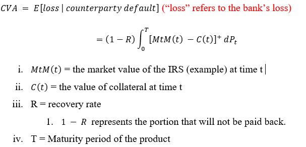
CVA – Credit Value Adjustment

CVA is the expected loss due to counterparty default. It accounts for the possibility that a counterparty may fail while the exposure is positive. Mathematically, it is the discounted expectation of exposure × loss-given-default × default probability. CVA became a regulatory requirement under Basel III and is the most widely known XVA component.

DVA – Debit Value Adjustment

DVA mirrors CVA but reflects the institution’s own default risk. If the bank itself defaults while the exposure is negative, this creates a gain from the perspective of the shareholder. While conceptually symmetric to CVA, DVA cannot usually be monetized, and its inclusion depends on accounting standards.

FVA – Funding Value Adjustment

FVA measures the cost of funding uncollateralized or partially collateralized positions.

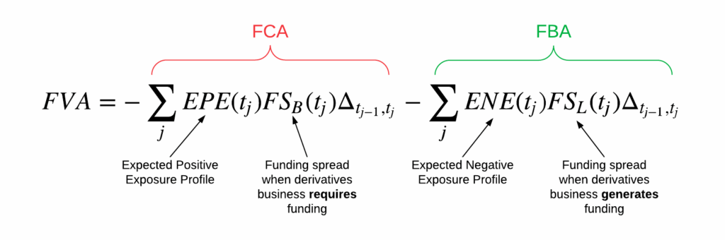
It arises from asymmetric borrowing and lending rates: funding a derivative generally requires borrowing at a spread above the risk-free rate, and this spread becomes part of the adjusted price. FVA is highly institution-specific, sensitive to treasury curves and liquidity policies.

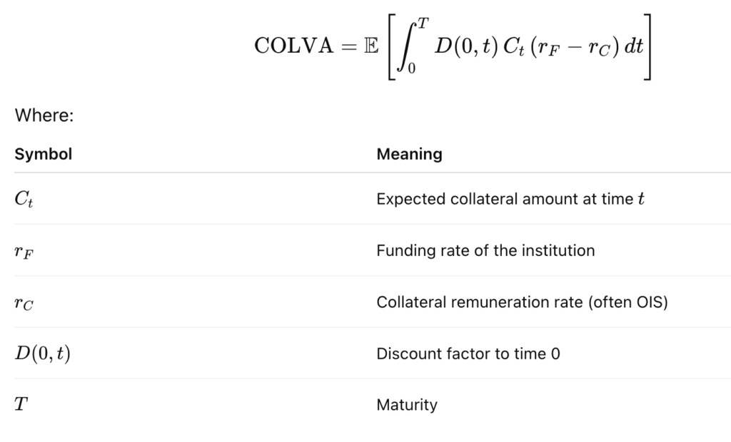
COLVA – Collateral Value Adjustment

COLVA captures the economic effect of posting or receiving collateral under a Credit Support Annex (CSA). It reflects the remuneration of the collateral account and the mechanics of discounting under different collateral currencies.

MVA – Margin Value Adjustment

MVA represents the cost of posting initial margin, particularly relevant for centrally cleared derivatives and uncleared margin rules. Since initial margin is locked up and earns little, MVA quantifies the funding drag associated with this constraint.

[math]
\large
\text{MVA} = -\int_0^T \mathbb{E}[\text{IM}(t)] , (f(t) – r(t)), dt.
[/math]

KVA – Capital Value Adjustment

KVA measures the cost of regulatory capital required to support the trade over its lifetime. Because capital is not free, banks incorporate a charge to account for the expected cost of holding capital against credit, market, and counterparty risk.

A commonly used representation of KVA is the discounted cost of holding regulatory capital K(t)K(t)K(t) over the life of the trade, multiplied by the bank’s hurdle rate hhh (the required return on capital):

[math]
\large
\text{KVA} = -\int_0^T D(t), h, K(t), dt
[/math]

where:

  • K(t) is the projected regulatory capital requirement at time t (e.g., CVA capital, market risk capital, counterparty credit risk capital),
  • h is the hurdle rate (often 8–12% depending on institution),
  • D(t) is the discount factor,
  • T is the maturity of the trade or portfolio.

2.The Mathematics of XVA

Mathematically, XVA extends the classical risk-neutral valuation framework by adding credit, funding, collateral, and capital effects directly into the pricing equation. The total adjusted value of a derivative is typically expressed as:

[math]
V_{\text{XVA}} = V_0 + \text{CVA} + \text{DVA} + \text{FVA} + \text{MVA} + \text{KVA} + \cdots
[/math]

where V0​ is the clean, risk-neutral price. Each adjustment is computed as an expectation under a measure consistent with the institution’s funding and collateral assumptions. CVA, for example, is the expected discounted loss from counterparty default.

Because these adjustments are interdependent, the pricing problem is no longer a simple additive correction to the clean value but a genuinely nonlinear one. Funding costs depend on expected exposures, exposures depend on default and collateral dynamics, and capital charges feed back through both. The full XVA calculation therefore takes the form of a fixed-point problem in which the adjusted value appears inside its own expectation. In practice, modern XVA desks solve this system using large-scale Monte Carlo simulations with backward induction, ensuring that all components—credit, funding, collateral, and capital—are computed consistently under the same modelling assumptions. This unified approach captures the true economic cost of trading and forms the mathematical backbone of XVA analytics in industry.

3.Calculate xVA in C++

To make the discussion concrete, we can wrap a simple XVA engine into a small, header-only C++ “library” that you can drop into an existing pricing codebase. The idea is to assume that exposure profiles and curves are already computed elsewhere (e.g. via a Monte Carlo engine) and focus on turning those into CVA, DVA, FVA, and KVA numbers along a time grid.

Below is a minimal example. It is not production-grade, but it shows the structure of a clean API that you can extend with your own models and data sources.

// xva.hpp
#pragma once
#include <vector>
#include <functional>
#include <numeric>

namespace xva {

struct Curve {
    // Discount factor P(0, t)
    std::function<double(double)> df;
};

struct SurvivalCurve {
    // Survival probability S(0, t)
    std::function<double(double)> surv;
};

struct XVAInputs {
    double V0;  // clean (risk-neutral) price

    Curve discount;
    SurvivalCurve counterpartySurv;
    SurvivalCurve firmSurv;

    std::vector<double> timeGrid;              // t_0, ..., t_N
    std::vector<double> expectedPositiveEE;    // EPE(t_i)
    std::vector<double> expectedNegativeEE;    // ENE(t_i)

    double lgdCounterparty; // 1 - recovery_C
    double lgdFirm;         // 1 - recovery_F
    double fundingSpread;   // flat funding spread (annualised)
    double capitalCharge;   // flat KVA multiplier (for illustration)
};

struct XVAResult {
    double V0;
    double cva;
    double dva;
    double fva;
    double kva;

    double total() const {
        return V0 + cva + dva + fva + kva;
    }
};

// Helper: simple forward finite difference for default density
inline double defaultDensity(const SurvivalCurve& S, double t0, double t1) {
    double s0 = S.surv(t0);
    double s1 = S.surv(t1);
    if (s0 <= 0.0) return 0.0;
    return (s0 - s1); // ΔQ ≈ S(t0) - S(t1)
}

inline XVAResult computeXVA(const XVAInputs& in) {
    const auto& t = in.timeGrid;
    const auto& EPE = in.expectedPositiveEE;
    const auto& ENE = in.expectedNegativeEE;

    double cva = 0.0;
    double dva = 0.0;
    double fva = 0.0;
    double kva = 0.0;

    std::size_t n = t.size();
    if (n < 2 || EPE.size() != n || ENE.size() != n)
        return {in.V0, 0.0, 0.0, 0.0, 0.0};

    for (std::size_t i = 0; i + 1 < n; ++i) {
        double t0 = t[i];
        double t1 = t[i + 1];

        double dt = t1 - t0;
        double dfMid = in.discount.df(0.5 * (t0 + t1));

        double dQcp = defaultDensity(in.counterpartySurv, t0, t1);
        double dQfm = defaultDensity(in.firmSurv,         t0, t1);

        double EPEmid = 0.5 * (EPE[i] + EPE[i+1]);
        double ENEmid = 0.5 * (ENE[i] + ENE[i+1]);

        // Simplified discretised formulas:
        cva += dfMid * in.lgdCounterparty * EPEmid * dQcp;
        dva -= dfMid * in.lgdFirm         * ENEmid * dQfm;

        // FVA and KVA: toy versions using EPE as proxy for funding/capital.
        fva -= dfMid * in.fundingSpread * EPEmid * dt;
        kva -= dfMid * in.capitalCharge * EPEmid * dt;
    }

    return {in.V0, cva, dva, fva, kva};
}

} // namespace xva

An example of usage:

#include "xva.hpp"
#include <cmath>
#include <iostream>

int main() {
    using namespace xva;

    XVAInputs in;
    in.V0 = 1.0; // clean price

    // Flat 2% discount curve
    in.discount.df = [](double t) {
        double r = 0.02;
        return std::exp(-r * t);
    };

    // Simple exponential survival with constant intensities
    double lambdaC = 0.01; // counterparty hazard
    double lambdaF = 0.005; // firm hazard

    in.counterpartySurv.surv = [lambdaC](double t) {
        return std::exp(-lambdaC * t);
    };
    in.firmSurv.surv = [lambdaF](double t) {
        return std::exp(-lambdaF * t);
    };

    // Time grid and toy exposure profiles
    int N = 10;
    in.timeGrid.resize(N + 1);
    in.expectedPositiveEE.resize(N + 1);
    in.expectedNegativeEE.resize(N + 1);

    for (int i = 0; i <= N; ++i) {
        double t = 0.5 * i; // every 6 months
        in.timeGrid[i] = t;

        // Toy exposures: decaying positive, small negative
        in.expectedPositiveEE[i] = std::max(0.0, 1.0 * std::exp(-0.1 * t));
        in.expectedNegativeEE[i] = -0.2 * std::exp(-0.1 * t);
    }

    in.lgdCounterparty = 0.6;
    in.lgdFirm         = 0.6;
    in.fundingSpread   = 0.01;
    in.capitalCharge   = 0.005;

    XVAResult res = computeXVA(in);

    std::cout << "V0  = " << res.V0  << "\n"
              << "CVA = " << res.cva << "\n"
              << "DVA = " << res.dva << "\n"
              << "FVA = " << res.fva << "\n"
              << "KVA = " << res.kva << "\n"
              << "V_XVA = " << res.total() << "\n";

    return 0;
}

This gives you:

  • A single header (xva.hpp) you can drop into your project.
  • A clean XVAInputs → XVAResult interface.
  • A place to plug in your own discount curves, survival curves, and exposure profiles from a more sophisticated engine.

You can then grow this skeleton (multi-curve setup, CSA terms, stochastic LGD, wrong-way risk, etc.) while keeping the same plug-and-play interface.

4.Conclusion

XVA has transformed derivative pricing from a clean, risk-neutral exercise into a fully integrated measure of economic value that accounts for credit, funding, collateral, and capital effects. The mathematical framework shows that these adjustments are not isolated add-ons but components of a coupled, nonlinear valuation problem. In practice, solving this system requires consistent modelling assumptions, carefully constructed exposure profiles, and scalable numerical methods.

The C++ snippet provided in the previous section illustrates how these ideas translate into a concrete, plug-and-play engine. Although simplified, it captures the essential workflow used on modern XVA desks: compute discounted exposures, combine them with survival probabilities and cost curves, and aggregate the resulting adjustments into a unified valuation.

As models evolve and regulatory requirements tighten, XVA will continue to shape how financial institutions assess the true cost of trading. A solid understanding of its mathematical foundations and computational techniques is therefore indispensable for quants and risk engineers looking to build accurate, scalable, and future-proof pricing systems.

November 16, 2025 0 comments
how to calculate Potential Future Exposure(PFE)?
Credit Risk

How to Calculate Potential Future Exposure (PFE)?

by Clement D. November 15, 2025

In modern investment banking, managing counterparty credit risk has become just as important as pricing the trade itself. Every derivative contract, from a simple interest rate swap to a complex cross-currency structure, carries the risk that the counterparty might default before the trade matures. When that happens, what really matters isn’t today’s mark-to-market, but what the exposure could be at the moment of default. That’s where Potential Future Exposure comes in: what is the Potential Future Exposure? How to calculate the Potential Future Exposure (PFE)?

How to Calculate Expected Exposure and Potential Future Exposure

1. What is the Potential Future Exposure(PFE)?

PFE quantifies the worst-case exposure a bank could face at a given confidence level and future time horizon. It doesn’t ask “what’s the average exposure?”, but rather “what’s the exposure in the 95th percentile scenario, one year from now?”. This risk-focused lens makes PFE a cornerstone of credit risk measurement, capital allocation, and pricing.

Before talking about PFE, we need to talk about mark-to-market (MtM), exposure end Expected Exposure (EE).

At any future time t, the exposure of a derivative or portfolio to a counterparty is defined as the positive mark-to-market (MtM) value from the bank’s perspective:

[math]\large E(t) = \max(V(t), 0)[/math]

where

  • [math]V(t)[/math] is the (random) value of the portfolio at time [math]t[/math],
  • [math]E(t)[/math] is the exposure — it cannot be negative, because if [math]V(t) < 0[/math], the exposure is zero (the counterparty owes you nothing).

The Expected Exposure (EE) at time [math]t[/math] is the expected value of that random exposure across all simulated market scenarios:

[math]\large EE(t) = \mathbb{E}\big[ E(t) \big][/math]

It represents the average positive exposure at time [math]t[/math].

You can see it like this:

This other chart shows how a portfolio’s current exposure evolves into a distribution of possible future exposures, with the Expected MtM as the mean, the Expected Exposure (EE) as the average of positive values, and the Potential Future Exposure (PFE) marking the high-confidence tail (worst-case exposure) of that distribution.

For a given future time t and confidence level [math] \alpha [/math], the Potential Future Exposure (PFE) is defined as such:

  • [math]E(t) = \max(V(t), 0)[/math] is the exposure,
  • [math]V(t)[/math] is the mark-to-market value of the portfolio at time [math]t[/math], and
  • [math]\alpha[/math] is the confidence level (e.g. 0.95 or 0.99).

we’re saying:

“Find the smallest value x such that the probability that exposure E(t) is below x is at least alpha.”

2. Why Does PFE Matter?

Potential Future Exposure (PFE) matters because it quantifies the worst-case credit exposure a bank could face with a counterparty at some point in the future. In essence, it asks: “How bad could it get?”

In trading, exposure today (the mark-to-market) is only a snapshot: what truly drives risk is how that exposure might evolve as markets move. PFE captures this by modeling thousands of potential future scenarios for rates, FX, equities, and credit spreads, and then measuring the high-percentile outcome (e.g. 95th or 99th).

Banks use PFE to set counterparty limits, ensuring that no single entity can cause unacceptable losses. Risk managers monitor these limits daily and reduce exposure through collateral, netting, or hedging.

PFE also feeds into regulatory capital frameworks such as Basel’s SA-CCR, influencing how much capital the bank must hold against derivative portfolios.

In trading desks, PFE affects pricing decisions: the higher the potential exposure, the higher the credit charge embedded in the trade price. Front-office, credit, and treasury teams all rely on PFE curves to understand how exposures behave over time and under stress.

In short, PFE transforms uncertain future risk into a measurable, actionable metric that connects market volatility, counterparty behavior, and balance-sheet safety — a critical pillar of counterparty credit risk management.

3. An Implementation in C++

Here’s a compact, production-style C++17 example that computes EE(t) and PFE(t, α) for a simple FX forward under GBM. It’s self-contained (only <random>, <vector>, etc.), and set up so you can swap in your own portfolio pricer later.

It simulates risk factor paths StS_tSt​, revalues the forward V(t)=N (St−K) DF(t)V(t)=N\,(S_t-K)\,DF(t)V(t)=N(St​−K)DF(t), takes exposure E(t)=max⁡(V(t),0)E(t)=\max(V(t),0)E(t)=max(V(t),0), then reports EE and PFE across a time grid.

// pfe_fx_forward.cpp
// C++17: Monte Carlo EE(t) and PFE(t, alpha) for an FX forward under GBM.

#include <algorithm>
#include <cmath>
#include <iomanip>
#include <iostream>
#include <numeric>
#include <random>
#include <string>
#include <vector>

// --------------------------- Utilities ---------------------------

// Quantile (0<alpha<1) of a vector (non-const because we sort).
double percentile(std::vector<double>& xs, double alpha) {
    if (xs.empty()) return 0.0;
    std::sort(xs.begin(), xs.end());
    // "linear interpolation between closest ranks" can be used;
    // here we do a simple nearest-rank with floor to be conservative for PFE.
    const double pos = alpha * (xs.size() - 1);
    const size_t idx = static_cast<size_t>(std::floor(pos));
    const double frac = pos - idx;
    if (idx + 1 < xs.size())
        return xs[idx] * (1.0 - frac) + xs[idx + 1] * frac;
    return xs.back();
}

// Discount factor assuming flat domestic rate r_d.
inline double discount(double r_d, double t) {
    return std::exp(-r_d * t);
}

// --------------------------- Model & Pricer ---------------------------

// Evolve FX under GBM: dS = S * ( (r_d - r_f) dt + sigma dW )
void simulate_paths_gbm(
    std::vector<std::vector<double>>& S, // [nPaths][nSteps+1]
    double S0, double r_d, double r_f, double sigma,
    double T, int nSteps, std::mt19937_64& rng)
{
    const double dt = T / nSteps;
    std::normal_distribution<double> Z(0.0, 1.0);

    for (size_t p = 0; p < S.size(); ++p) {
        S[p][0] = S0;
        for (int j = 1; j <= nSteps; ++j) {
            const double z = Z(rng);
            const double drift = (r_d - r_f - 0.5 * sigma * sigma) * dt;
            const double diff  = sigma * std::sqrt(dt) * z;
            S[p][j] = S[p][j - 1] * std::exp(drift + diff);
        }
    }
}

// Simple FX forward MtM from bank's perspective at time t:
// V(t) = N * ( S(t) - K ) * DF_d(t)
// (Domestic-discounted payoff; sign assumes receiving S, paying K at T.)
// If you want precise forward maturing at T, you can scale by DF(T)/DF(t)
// and/or set value only at maturity; here we keep a running MtM proxy.
inline double forward_mtm(double notional, double S_t, double K, double r_d, double t) {
    return notional * (S_t - K) * discount(r_d, t);
}

// Exposure is positive part of MtM.
inline double exposure(double Vt) { return std::max(Vt, 0.0); }

// --------------------------- Main EE/PFE Engine ---------------------------

struct Results {
    std::vector<double> times;     // size nSteps+1
    std::vector<double> EE;        // Expected Exposure at each time
    std::vector<double> PFE;       // Potential Future Exposure at each time
};

Results compute_EE_PFE_FXForward(
    int nPaths, int nSteps, double T,
    double S0, double r_d, double r_f, double sigma,
    double notional, double strikeK,
    double alpha, uint64_t seed = 42ULL)
{
    // 1) Simulate FX paths
    std::mt19937_64 rng(seed);
    std::vector<std::vector<double>> S(nPaths, std::vector<double>(nSteps + 1));
    simulate_paths_gbm(S, S0, r_d, r_f, sigma, T, nSteps, rng);

    // 2) Time grid
    std::vector<double> times(nSteps + 1);
    for (int j = 0; j <= nSteps; ++j) times[j] = (T * j) / nSteps;

    // 3) For each time, compute exposures across paths, then EE and PFE
    std::vector<double> EE(nSteps + 1, 0.0);
    std::vector<double> PFE(nSteps + 1, 0.0);
    std::vector<double> bucket(nPaths);

    for (int j = 0; j <= nSteps; ++j) {
        const double t = times[j];

        // Build exposure samples at time t across paths
        for (int p = 0; p < nPaths; ++p) {
            const double Vt = forward_mtm(notional, S[p][j], strikeK, r_d, t);
            bucket[p] = exposure(Vt);
        }

        // EE(t) = mean of positive exposures
        const double sum = std::accumulate(bucket.begin(), bucket.end(), 0.0);
        EE[j] = sum / static_cast<double>(nPaths);

        // PFE(t, alpha) = alpha-quantile of exposures
        // (we make a working copy because percentile sorts in-place)
        std::vector<double> tmp = bucket;
        PFE[j] = percentile(tmp, alpha);
    }

    return { std::move(times), std::move(EE), std::move(PFE) };
}

// --------------------------- Demo / CLI ---------------------------

int main(int argc, char** argv) {
    // Default parameters (override via argv if desired).
    int    nPaths  = 20000;
    int    nSteps  = 20;         // e.g., quarterly over 5 years => set T=5.0 and nSteps=20
    double T       = 2.0;        // years
    double S0      = 1.10;       // spot FX (e.g., USD per EUR)
    double r_d     = 0.035;      // domestic rate
    double r_f     = 0.015;      // foreign rate
    double sigma   = 0.12;       // FX vol
    double N       = 10'000'000; // notional
    double K       = 1.12;       // forward strike
    double alpha   = 0.95;       // PFE quantile
    uint64_t seed  = 42ULL;

    // (Optional) basic CLI parsing for quick tweaks
    if (argc > 1) nPaths = std::stoi(argv[1]);
    if (argc > 2) nSteps = std::stoi(argv[2]);
    if (argc > 3) T      = std::stod(argv[3]);

    auto res = compute_EE_PFE_FXForward(
        nPaths, nSteps, T, S0, r_d, r_f, sigma, N, K, alpha, seed
    );

    // Pretty print
    std::cout << std::fixed << std::setprecision(6);
    std::cout << "t,EE,PFE\n";
    for (size_t j = 0; j < res.times.size(); ++j) {
        std::cout << res.times[j] << "," << res.EE[j] << "," << res.PFE[j] << "\n";
    }

    // A quick sanity summary at T/2 and T
    auto halfway = res.times.size() / 2;
    std::cout << "\nSummary\n";
    std::cout << "EE(T/2)  = " << res.EE[halfway] << "\n";
    std::cout << "PFE(T/2) = " << res.PFE[halfway] << "\n";
    std::cout << "EE(T)    = " << res.EE.back() << "\n";
    std::cout << "PFE(T)   = " << res.PFE.back() << "\n";

    return 0;
}

3. Explanation of the Code

So, how to calculate the Pontential Future Exposure(PFE)? This C++ program demonstrates how to estimate Expected Exposure (EE) and Potential Future Exposure (PFE) using a simple Monte Carlo engine for an FX forward.

It begins by simulating many potential future FX rate paths under a Geometric Brownian Motion (GBM) model, where each path represents how the exchange rate might evolve given drift, volatility, and random shocks. For every time step, the program computes the mark-to-market (MtM) of the FX forward as the discounted notional times the difference between simulated spot and strike.

For every time step, the program computes the mark-to-market (MtM) of the FX forward as the discounted notional times the difference between simulated spot and strike. Negative MtM values imply the bank owes the counterparty, so exposures are floored at zero using max(Vt, 0). Across all paths, the program averages these exposures to get the Expected Exposure EE(t) and extracts the high-quantile value to obtain PFE(t, α): the 95th percentile exposure. It iterates this process across the time grid to build the full exposure profile. The simulation uses <random> for Gaussian draws, std::vector containers for efficiency, and a clean modular structure separating simulation, pricing, and analytics. Finally, results are printed as a CSV table of time, EE, and PFE, ready for plotting or integration into a larger risk system.

4. What are the key parameters driving the PFE value?

PFE is not a static number: it’s shaped by a mix of market dynamics, trade structure, and risk mitigation terms.
At its core, it reflects how volatile and directional the portfolio’s mark-to-market (MtM) could become under plausible future scenarios.
The main drivers are:

a. Market Volatility (σ)
The higher the volatility of the underlying risk factors (interest rates, FX, equities, credit spreads), the wider the future distribution of MtM values.
Since PFE is a high quantile of that distribution, higher volatility directly pushes PFE up.

b. Time Horizon (t)
Exposure uncertainty compounds over time.
The longer the time horizon, the more potential market moves accumulate, leading to a larger spread of outcomes and therefore higher PFE.

c. Product Type and Optionality
Linear products (like forwards or swaps) have exposures that evolve predictably, while nonlinear products (like options) exhibit asymmetric exposure.
For example, an option seller’s exposure can explode if volatility rises, so the product payoff shape strongly affects the PFE profile.

d. Counterparty Netting Set
If multiple trades exist under the same netting agreement, positive and negative MtMs offset each other.
A large, well-balanced netting set reduces overall exposure variance and therefore lowers PFE.

e. Collateralization / CSA Terms
Credit Support Annex (CSA) terms (thresholds, minimum transfer amounts, margin frequency): they determine how much exposure remains unsecured.
Frequent margining and low thresholds sharply reduce PFE; loose or infrequent margining increases it

f. Correlation and Wrong-Way Risk
If the exposure tends to rise when the counterparty’s credit worsens (e.g. a borrower correlated with its asset), this wrong-way risk amplifies effective PFE because losses are more likely when the counterparty defaults

g. Interest Rate Differentials and Discounting
In FX and IR products, differences between domestic and foreign rates (or curve shapes) affect the drift of MtM paths.
Higher discount rates reduce future MtMs and hence lower PFE in present-value terms

h. Confidence Level (α)
By definition, PFE depends on the percentile you choose: 95%, 97.5%, or 99%.
A higher confidence level means a deeper tail cut and therefore a higher PFE.

November 15, 2025 0 comments
tree shap model
Credit Risk

Attribution Modeling for Credit PnL Using TreeSHAP

by Clement D. September 6, 2024

In modern credit trading, understanding why PnL moves is just as important as tracking that it moved.
When billions of data points flow through trading systems daily, intuition and heuristics fall short.
This article presents a scalable method for attributing PnL changes to specific credit risk drivers.
We model feature deltas — changes in exposure, spreads, and counterparty metrics — across time.


We train a LightGBM model to learn nonlinear relationships between deltas and ΔPnL.
Then, we apply TreeSHAP to extract the top features responsible for each credit-related PnL movement.
The result is a transparent, auditable, per-entity view of what caused the last PnL move.
This is not prediction, it’s attribution — a diagnostic engine for credit risk.

1. Introduction: The Need for Attribution, Not Prediction

Credit-related PnL refers to profit and loss driven by credit risk exposure — such as changes in counterparty credit spreads, rating downgrades, or shifts in default probabilities.
It captures the financial impact of events like widening CDS, growing exposures, or collateral changes, rather than market or operational effects.


For traders, a sudden loss tied to a counterparty matters less than knowing which risk factor caused it.
For quants, understanding nonlinear relationships between inputs and PnL is key to model trust and validation.
And for risk teams, attribution supports regulatory reporting, stress testing, and early warnings.
But with data at the scale of billions of deltas, traditional methods fail to offer clear answers.
We propose a hybrid pipeline: use Python to train a LightGBM model on feature deltas and PnL deltas.
Then apply TreeSHAP to explain which deltas caused most of the PnL movement.
For real-time inference, we port the model and SHAP logic to a high-performance C++ backend.
The result: an explainable, scalable, and production-ready system for credit PnL attribution at scale.

2. Data Design: Tracking the Right Deltas

Every 15 minutes, a new snapshot arrives — a high-dimensional vector (10,000+ features) representing the full state of the trading system: exposure, spreads, counterparty credit ratings, margin calls, instrument properties, and more.

This raw data isn’t yet meaningful. To extract signal, we compute deltas: changes in features between consecutive time windows. These represent what moved.

Alongside the feature deltas, we compute the PnL delta, giving us a supervised signal to explain: what caused the profit or loss change since the last window?

We filter and engineer meaningful features — credit spreads, counterparty ratings, net exposure, sector-level aggregates — to reduce noise and emphasize credit drivers.

Using deltas instead of raw levels is key. Most credit features are auto-correlated or slow-moving — a high exposure value tells us less than a sudden increase in exposure.

The delta of a credit spread or notional tells us more about risk events, decisions, or systemic shifts than the absolute value alone.

By modeling dPnL ~ Δ_features, we move from static snapshots to causal attribution.

📄 Mocked Extract of Delta Dataset

timestampentityΔ_exposureΔ_cds_bnpΔ_rating_scoreΔ_sector_riskΔPnL
2025-06-23 10:00:00trader_01+2.3M+0.018-1+0.07-4.21M
2025-06-23 10:15:00trader_01-1.1M-0.0050-0.03+2.73M
2025-06-23 10:30:00trader_01+0.4M+0.00200-1.00M
  • Δ_exposure: Notional delta to counterparties
  • Δ_cds_bnp: Change in BNP CDS (in decimal)
  • Δ_rating_score: Discrete rating movement (e.g., 1 = downgrade)
  • Δ_sector_risk: Change in weighted average sector risk score
  • dPnL: Total change in credit-related PnL

We will drastically increase the dimensionality of those with 10k columns and 1 million rows.

We generate millions of entries in “delta_features.csv” and millions of delta PnLs in “delta_pnl.csv”

3. Modeling: Training a Gradient Boosted Tree on Deltas

To prepare for TreeSHAP attribution in this credit delta → PnL delta setup, you’ll want to use a LightGBM regression model that emphasizes explainability, stability, and performance.

✅ Goal:

  • Train a LightGBM model (Δfeatures → ΔPnL)
  • Export the model (model.txt)
  • Optionally export samples for testing C++ inference

🧠 File: train_model.py


import lightgbm as lgb
import pandas as pd

# Load delta feature and delta PnL data
X = pd.read_csv("delta_features.csv")
y = pd.read_csv("delta_pnl.csv")

# Train model
params = {
    "objective": "regression",
    "metric": "rmse",
    "learning_rate": 0.03,
    "num_leaves": 64,
    "feature_fraction": 0.6,
    "bagging_fraction": 0.8,
    "bagging_freq": 5,
    "lambda_l1": 0.1,
    "lambda_l2": 1.0,
    "min_data_in_leaf": 50,
    "verbose": -1
}
model = lgb.train(lgb.Dataset(X, label=y), params, num_boost_round=200)

# Save model
model.save_model("model.txt")

# Export a row (e.g., for test inference)
row_index = 12345
X.iloc[[row_index]].to_csv("sample_row.csv", index=False)
y.iloc[[row_index]].to_csv("sample_label.csv", index=False)

Then we can run the inferrence:

import pandas as pd
import shap
import lightgbm as lgb

# Load model and data
model = lgb.Booster(model_file="model.txt")          # Trained LGBM model
X = pd.read_csv("sample_row.csv")         # Latest 15-min features (deltas)
y_pnl = pd.read_csv("sample_label.csv")          # Actual PnL deltas (optional)

# Run SHAP
explainer = shap.TreeExplainer(model)
shap_values = explainer.shap_values(X)

# For a specific row (e.g. last 15-min observation)
row = 0
shap_row = shap_values[row]

# Create attribution table
explained = pd.DataFrame({
    "feature": X.columns,
    "shap_value": shap_row,
    "feature_value": X.iloc[row]
}).sort_values(by="shap_value", key=abs, ascending=False)

# Add cumulative contribution
explained["cum_impact"] = explained["shap_value"].cumsum()
total_impact = abs(explained["shap_value"]).sum()
explained["cum_percent"] = abs(explained["shap_value"]).cumsum() / total_impact

# Output: top features responsible for 90% of the PnL move
top_contributors = explained[explained["cum_percent"] <= 0.9]
print(top_contributors)

4. Results

📦 Output Example

      feature      shap_value  feature_value  cum_impact  cum_percent
23 spread_delta 0.68 12.0 0.68 0.42
14 curve_1y 0.51 3.2 1.19 0.72
9 exposure_bond 0.33 54.1 1.52 0.92

This shows:

  • The features most responsible for the ΔPnL for that 15-min slice
  • Their raw SHAP impact
  • How much of the total impact they cumulatively explain

September 6, 2024 0 comments

@2025 - All Right Reserved.


Back To Top
  • Home
  • News
  • Contact
  • About