Risk

Credit Valuation Adjustment (CVA) is the adjustment applied to a derivative’s default-free value to account for this counterparty credit risk. In simple terms, CVA is the present value of the expected loss caused by the possibility that the counterparty defaults while the derivative has positive exposure.

1. Understand the CVA Formula

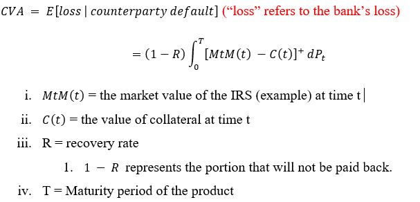
The term CVA (Credit Valuation Adjustment) is defined as:

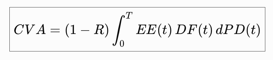
The discretized version of that integral is a sum:

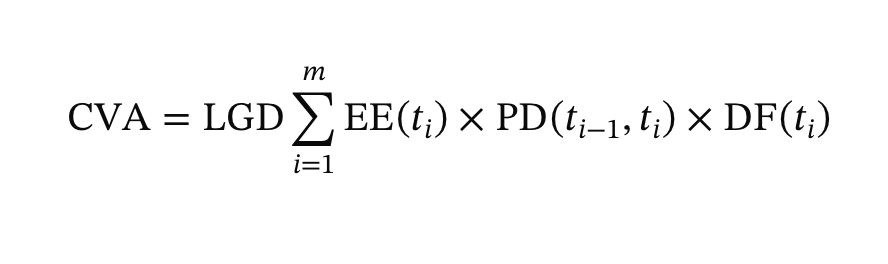
Credit Valuation Adjustment (CVA) Components

• LGD (Loss Given Default): The percentage of exposure lost if the counterparty defaults (1 – Recovery Rate).
• EE (Expected Exposure): The average positive value or market exposure of the portfolio at future time \(t_{i}\).
• PD (Probability of Default): The marginal chance that the counterparty defaults during the specific time interval.
• DF (Discount Factor): The present value factor that discounts future cash flows back to today.
• R (Recovery Rate) is the recovery rate of the counterparty.

A way to explain it is: at every future date, ask how much we could lose, how likely the counterparty is to default during that period, and what that loss is worth today.

Then add everything up.

First divide the life of the portfolio into dates:

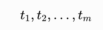
For all of those, it’s possible to calculate the Expected Exposure (EE). If the derivative has positive value, the counterparty owes you money and you are exposed to their default:

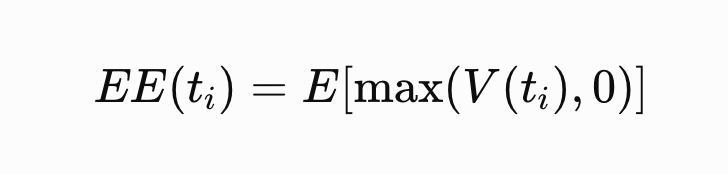
This is often obtained by simulating market variables such as interest rates, FX rates, equity prices, etc.

For example:

Why?
If the counterparty defaults when they owe you nothing, there is essentially no credit loss. CVA therefore depends on the amount you expect to be exposed to at the time of default.

For a real portfolio, this calculation should also reflect things such as netting and collateral.

Next calculate:

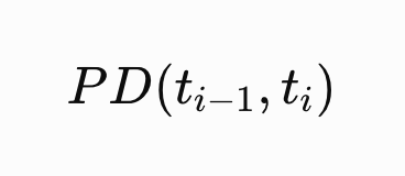
This is the probability that the counterparty survives until ti−1​ and then defaults between ti−1​ and ti​.

For example:

An important point is that we use the incremental default probability, not simply the cumulative probability of default by each year.

Why?
Default can only happen once. Each interval represents a different possible default time, so we want the probability that default occurs specifically in that interval.

Now apply LGD (Loss Given Default): if the counterparty defaults, you do not necessarily lose the entire exposure.

For example, if the assumed recovery rate is 40%: LGD=1−0.40=60%

If exposure at default is £10m: Expected loss if default occurs=10m×60%=£6m

Why?
Some money may be recovered through bankruptcy proceedings, collateral, restructuring, etc. CVA should measure the expected economic loss, rather than assuming a 100% loss.

But a loss occurring several years from now is not worth the same amount as a loss today.

So multiply by:

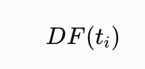
For example, if the 3-year discount factor is 0.92: £1m expected loss in year 3→£0.92m present value

Why?
CVA is a present-value adjustment to the value of the derivative today.

So, for each interval, we can calculate:

And finally sum across all periods:

Which can be summarized as:

Which is very close to the definition of expected loss:

2. How does CVA reduce the value of a derivative?

Credit Valuation Adjustment or CVA is not just a risk metric. It is a pricing adjustment that reflects the possibility that the counterparty may default before paying everything it owes.

Consider the derivative from the bank’s perspective.

If the derivative has a positive mark-to-market value, it is an asset for the bank: the counterparty owes money to the bank. If the counterparty defaults at that point, the bank may recover only part of that amount.

If the derivative has a negative mark-to-market value, the bank owes money to the counterparty instead. From the perspective of unilateral CVA, this does not create a loss from the counterparty’s default. This is why CVA focuses on positive exposure.

Suppose a derivative has a risk-free value of £10 million. If the counterparty were guaranteed never to default, the bank could value the derivative at the full £10 million.

Now suppose the present value of the expected loss caused by possible counterparty default is £300,000. That expected loss is the CVA.

The credit-adjusted value of the derivative becomes:

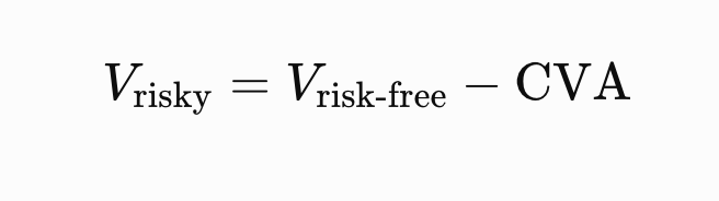
The derivative is worth less because some of its future positive cash flows may never actually be received.

This also explains why two otherwise identical derivatives may have different values when traded with different counterparties. A £10 million receivable from a highly creditworthy counterparty is more valuable than a £10 million receivable from a counterparty with a significant probability of default.

CVA provides a way to incorporate that difference directly into the valuation.

The relationship also gives some useful intuition: PD↑⇒CVA↑⇒Vrisky​↓

If the counterparty becomes more likely to default, CVA increases and the derivative becomes less valuable.

Similarly: EE↑⇒CVA↑⇒Vrisky​↓

If the bank expects to be owed more money in the future, more value is at risk if the counterparty defaults.

Conversely, better collateralisation, stronger netting agreements or an improvement in the counterparty’s credit quality can reduce expected losses and therefore reduce CVA.

So the key idea is simple:

CVA is the monetary value of counterparty credit risk embedded in the price of the derivative.

3. Implementation in C++

There are several ways to implement a CVA calculation in C++, depending on how much of the pricing stack you want to build yourself.

At the simplest level, you can assume that the expected exposure profile, default probabilities and discount factors have already been calculated. CVA then becomes a straightforward aggregation: CVA=LGDi∑​EE(ti​)×PD(ti−1​,ti​)×DF(ti​)

This is a good starting point because it isolates the CVA calculation from the more complex problem of generating future exposures.

A more complete implementation would typically involve one of the following approaches:

• Precomputed exposure profiles — read EE, PD and discount curves from upstream systems and aggregate them. This is the simplest approach.
• Monte Carlo simulation — simulate future market states, reprice the portfolio at each future date, and estimate EE(t) from the resulting exposure distribution.
• QuantLib — use existing pricing engines, yield curves, credit curves and stochastic processes rather than implementing every component from scratch.
• Production CVA engine — combine trade pricing, netting sets, collateral agreements, market simulation, credit curves and aggregation across thousands or millions of trades.

For illustration, we can start with the first approach.

Suppose the expected exposure profile is:

Year EE Incremental PD DF
1 10.0m 1.0% 0.97
2 14.0m 1.2% 0.94
3 8.0m 1.4% 0.91

A simple C++ implementation is then:

#include <iostream>
#include <vector>
#include <stdexcept>

struct CVAPoint {
    double expectedExposure;
    double defaultProbability;
    double discountFactor;
};

double calculateCVA(
    const std::vector<CVAPoint>& profile,
    double recoveryRate)
{
    if (recoveryRate < 0.0 || recoveryRate > 1.0) {
        throw std::invalid_argument("Invalid recovery rate");
    }

    const double lgd = 1.0 - recoveryRate;

    double cva = 0.0;

    for (const auto& point : profile) {
        cva += point.expectedExposure
             * point.defaultProbability
             * point.discountFactor
             * lgd;
    }

    return cva;
}

int main()
{
    std::vector<CVAPoint> profile = {
        {10'000'000.0, 0.010, 0.97},
        {14'000'000.0, 0.012, 0.94},
        { 8'000'000.0, 0.014, 0.91}
    };

    const double recoveryRate = 0.40;

    const double cva = calculateCVA(profile, recoveryRate);

    std::cout << "CVA = £" << cva << '\n';
}

For the first year, for example: 10,000,000×0.01×0.97×0.60=58,200

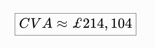
The three contributions are approximately: 58,200+94,752+61,152=214,104

so the resulting CVA is approximately:

4. CVA as part of the XVA framework

CVA is one component of the broader XVA framework used to adjust the clean, or risk-free, value of a derivative for costs and risks that are not captured by the classical pricing model.

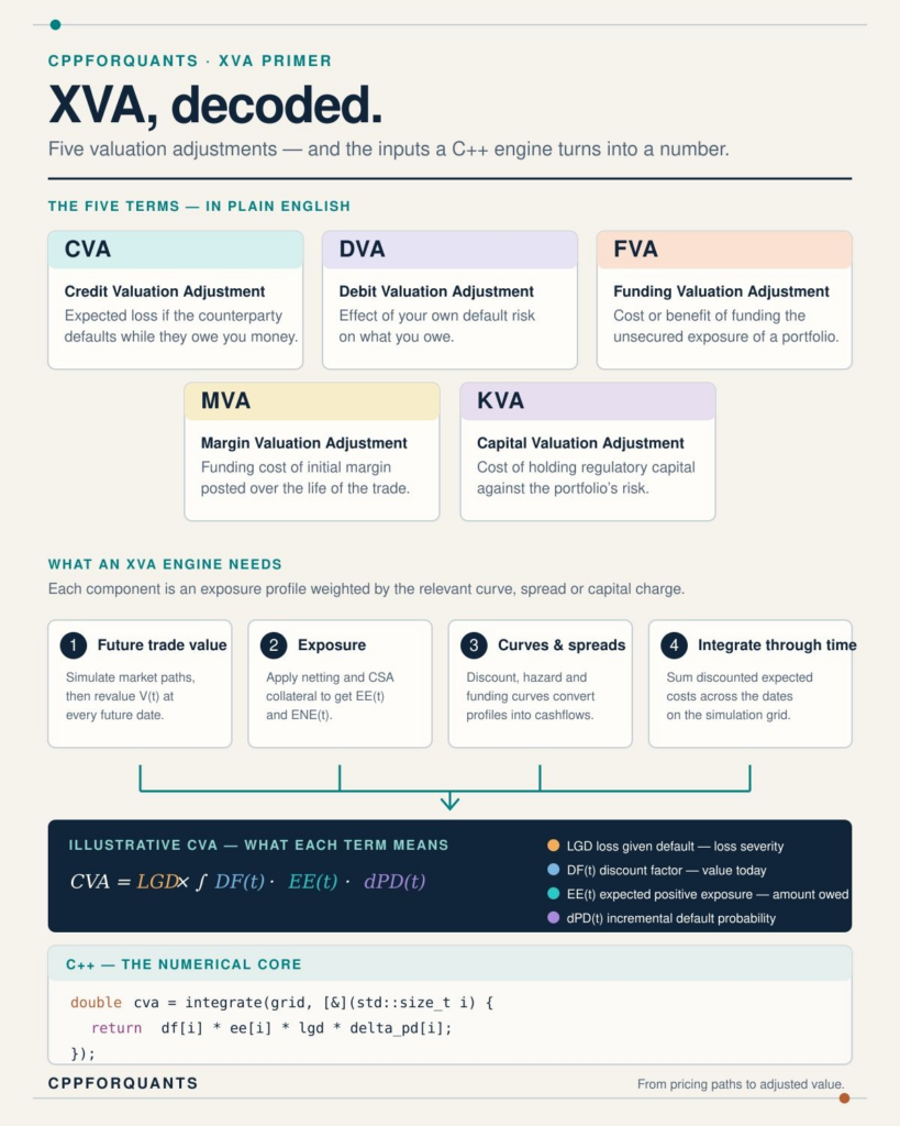
A useful way to think about the XVA stack is:

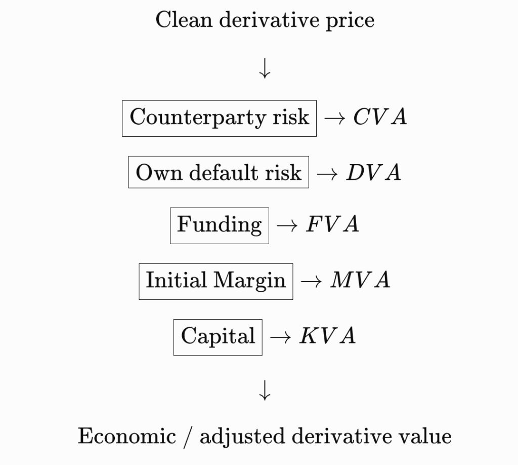
This is why CVA should not be viewed as an isolated calculation. It is one part of a much larger framework used by banks to determine the true economic cost of entering into and maintaining a derivative position.

It also explains why the same exposure simulation infrastructure can often support several XVA calculations. Once a system can simulate future portfolio values, collateral and exposure distributions, those simulations can be reused to calculate CVA, DVA, FVA, MVA and other adjustments.

In practice, this is one of the reasons XVA systems can become computationally demanding: a large bank may need to simulate future market states and reprice millions of trades across thousands of counterparties and many future time steps before the different valuation adjustments can be calculated.

5. 10 interview questions about CVA

1. What is CVA?
CVA is the credit valuation adjustment made to a derivative’s value to account for the possibility that the counterparty defaults.

2. Why does CVA reduce a derivative’s value?
Because a positive future payoff is worth less if there is a chance the counterparty will not fully pay it.

3. What is expected exposure?
Expected exposure is the average amount the bank expects to be owed by the counterparty at a future date.

4. What is the difference between EE and PFE?
EE is the average future exposure, while PFE measures a high percentile of potential exposure and focuses more on tail risk.

5. Where do default probabilities come from?
They are generally derived from the counterparty’s credit curve, often using CDS or bond market information.

6. Why use incremental default probabilities?
Because CVA needs the probability that default occurs within each specific time period, without double-counting default risk.

7. How do netting and collateral affect CVA?
They reduce the amount exposed to counterparty default and therefore generally reduce CVA.

8. What is wrong-way risk?
Wrong-way risk occurs when exposure increases at the same time as the counterparty becomes more likely to default.

9. How is CVA calculated with Monte Carlo simulation?
Future market scenarios are simulated, the portfolio is repriced, exposures are calculated, and the resulting expected losses are aggregated.

10. How does CVA fit into XVA?
CVA is the counterparty-credit component of XVA, alongside adjustments for own credit risk, funding, margin and capital costs.

What’s XVA? In modern derivative pricing, that question sits at the heart of almost every trading, risk, and regulatory discussion. XVA, short for X-Value Adjustments, refers to the suite of valuation corrections applied on top of a risk-neutral price to reflect credit risk, funding costs, collateral effects, and regulatory capital requirements. After the 2008 financial crisis, these adjustments evolved from a theoretical curiosity to a cornerstone of real-world derivative valuation.

Banks today do not quote the “clean” price of a swap or option alone; they quote an XVA-adjusted price. Whether the risk comes from counterparty default (CVA), a bank’s own credit (DVA), collateral remuneration (COLVA), the cost of funding uncollateralized trades (FVA), regulatory capital (KVA), or initial margin requirements (MVA), XVA brings all these effects together under a consistent mathematical and computational framework.

1.What is XVA? The XVA Family

XVA is a collective term for the suite of valuation adjustments applied to the theoretical, risk-neutral price of a derivative to reflect real-world constraints such as credit risk, funding costs, collateralization, and regulatory capital. In practice, the price a bank shows to a client is not the pure model price but the XVA-adjusted price, which embeds all these effects into a unified framework.

Modern XVA desks typically decompose the total adjustment into several components, each capturing a specific economic cost or risk. Together, they form the XVA family:

CVA – Credit Value Adjustment

CVA is the expected loss due to counterparty default. It accounts for the possibility that a counterparty may fail while the exposure is positive. Mathematically, it is the discounted expectation of exposure × loss-given-default × default probability. CVA became a regulatory requirement under Basel III and is the most widely known XVA component.

DVA – Debit Value Adjustment

DVA mirrors CVA but reflects the institution’s own default risk. If the bank itself defaults while the exposure is negative, this creates a gain from the perspective of the shareholder. While conceptually symmetric to CVA, DVA cannot usually be monetized, and its inclusion depends on accounting standards.

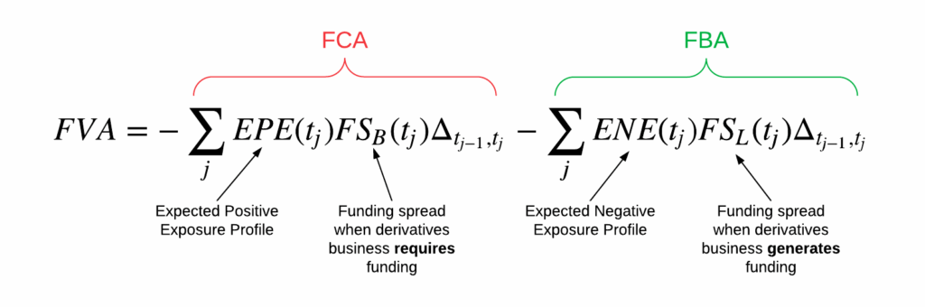
FVA – Funding Value Adjustment

FVA measures the cost of funding uncollateralized or partially collateralized positions.

It arises from asymmetric borrowing and lending rates: funding a derivative generally requires borrowing at a spread above the risk-free rate, and this spread becomes part of the adjusted price. FVA is highly institution-specific, sensitive to treasury curves and liquidity policies.

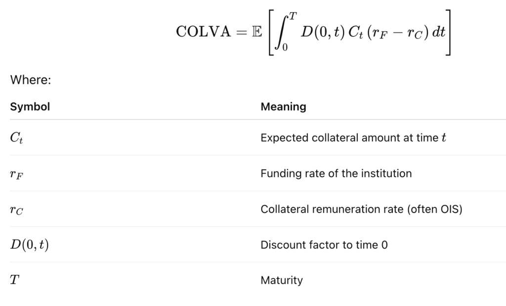
COLVA – Collateral Value Adjustment

COLVA captures the economic effect of posting or receiving collateral under a Credit Support Annex (CSA). It reflects the remuneration of the collateral account and the mechanics of discounting under different collateral currencies.

MVA – Margin Value Adjustment

MVA represents the cost of posting initial margin, particularly relevant for centrally cleared derivatives and uncleared margin rules. Since initial margin is locked up and earns little, MVA quantifies the funding drag associated with this constraint.

[math]
\large
\text{MVA} = -\int_0^T \mathbb{E}[\text{IM}(t)] , (f(t) – r(t)), dt.
[/math]

KVA – Capital Value Adjustment

KVA measures the cost of regulatory capital required to support the trade over its lifetime. Because capital is not free, banks incorporate a charge to account for the expected cost of holding capital against credit, market, and counterparty risk.

A commonly used representation of KVA is the discounted cost of holding regulatory capital K(t)K(t)K(t) over the life of the trade, multiplied by the bank’s hurdle rate hhh (the required return on capital):

[math]
\large
\text{KVA} = -\int_0^T D(t), h, K(t), dt
[/math]

where:

• K(t) is the projected regulatory capital requirement at time t (e.g., CVA capital, market risk capital, counterparty credit risk capital),
• h is the hurdle rate (often 8–12% depending on institution),
• D(t) is the discount factor,
• T is the maturity of the trade or portfolio.

2.The Mathematics of XVA

Mathematically, XVA extends the classical risk-neutral valuation framework by adding credit, funding, collateral, and capital effects directly into the pricing equation. The total adjusted value of a derivative is typically expressed as:

[math]
V_{\text{XVA}} = V_0 + \text{CVA} + \text{DVA} + \text{FVA} + \text{MVA} + \text{KVA} + \cdots
[/math]

where V0​ is the clean, risk-neutral price. Each adjustment is computed as an expectation under a measure consistent with the institution’s funding and collateral assumptions. CVA, for example, is the expected discounted loss from counterparty default.

Because these adjustments are interdependent, the pricing problem is no longer a simple additive correction to the clean value but a genuinely nonlinear one. Funding costs depend on expected exposures, exposures depend on default and collateral dynamics, and capital charges feed back through both. The full XVA calculation therefore takes the form of a fixed-point problem in which the adjusted value appears inside its own expectation. In practice, modern XVA desks solve this system using large-scale Monte Carlo simulations with backward induction, ensuring that all components—credit, funding, collateral, and capital—are computed consistently under the same modelling assumptions. This unified approach captures the true economic cost of trading and forms the mathematical backbone of XVA analytics in industry.

3.Calculate xVA in C++

To make the discussion concrete, we can wrap a simple XVA engine into a small, header-only C++ “library” that you can drop into an existing pricing codebase. The idea is to assume that exposure profiles and curves are already computed elsewhere (e.g. via a Monte Carlo engine) and focus on turning those into CVA, DVA, FVA, and KVA numbers along a time grid.

Below is a minimal example. It is not production-grade, but it shows the structure of a clean API that you can extend with your own models and data sources.

// xva.hpp
#pragma once
#include <vector>
#include <functional>
#include <numeric>

namespace xva {

struct Curve {
    // Discount factor P(0, t)
    std::function<double(double)> df;
};

struct SurvivalCurve {
    // Survival probability S(0, t)
    std::function<double(double)> surv;
};

struct XVAInputs {
    double V0;  // clean (risk-neutral) price

    Curve discount;
    SurvivalCurve counterpartySurv;
    SurvivalCurve firmSurv;

    std::vector<double> timeGrid;              // t_0, ..., t_N
    std::vector<double> expectedPositiveEE;    // EPE(t_i)
    std::vector<double> expectedNegativeEE;    // ENE(t_i)

    double lgdCounterparty; // 1 - recovery_C
    double lgdFirm;         // 1 - recovery_F
    double fundingSpread;   // flat funding spread (annualised)
    double capitalCharge;   // flat KVA multiplier (for illustration)
};

struct XVAResult {
    double V0;
    double cva;
    double dva;
    double fva;
    double kva;

    double total() const {
        return V0 + cva + dva + fva + kva;
    }
};

// Helper: simple forward finite difference for default density
inline double defaultDensity(const SurvivalCurve& S, double t0, double t1) {
    double s0 = S.surv(t0);
    double s1 = S.surv(t1);
    if (s0 <= 0.0) return 0.0;
    return (s0 - s1); // ΔQ ≈ S(t0) - S(t1)
}

inline XVAResult computeXVA(const XVAInputs& in) {
    const auto& t = in.timeGrid;
    const auto& EPE = in.expectedPositiveEE;
    const auto& ENE = in.expectedNegativeEE;

    double cva = 0.0;
    double dva = 0.0;
    double fva = 0.0;
    double kva = 0.0;

    std::size_t n = t.size();
    if (n < 2 || EPE.size() != n || ENE.size() != n)
        return {in.V0, 0.0, 0.0, 0.0, 0.0};

    for (std::size_t i = 0; i + 1 < n; ++i) {
        double t0 = t[i];
        double t1 = t[i + 1];

        double dt = t1 - t0;
        double dfMid = in.discount.df(0.5 * (t0 + t1));

        double dQcp = defaultDensity(in.counterpartySurv, t0, t1);
        double dQfm = defaultDensity(in.firmSurv,         t0, t1);

        double EPEmid = 0.5 * (EPE[i] + EPE[i+1]);
        double ENEmid = 0.5 * (ENE[i] + ENE[i+1]);

        // Simplified discretised formulas:
        cva += dfMid * in.lgdCounterparty * EPEmid * dQcp;
        dva -= dfMid * in.lgdFirm         * ENEmid * dQfm;

        // FVA and KVA: toy versions using EPE as proxy for funding/capital.
        fva -= dfMid * in.fundingSpread * EPEmid * dt;
        kva -= dfMid * in.capitalCharge * EPEmid * dt;
    }

    return {in.V0, cva, dva, fva, kva};
}

} // namespace xva

An example of usage:

#include "xva.hpp"
#include <cmath>
#include <iostream>

int main() {
    using namespace xva;

    XVAInputs in;
    in.V0 = 1.0; // clean price

    // Flat 2% discount curve
    in.discount.df = [](double t) {
        double r = 0.02;
        return std::exp(-r * t);
    };

    // Simple exponential survival with constant intensities
    double lambdaC = 0.01; // counterparty hazard
    double lambdaF = 0.005; // firm hazard

    in.counterpartySurv.surv = [lambdaC](double t) {
        return std::exp(-lambdaC * t);
    };
    in.firmSurv.surv = [lambdaF](double t) {
        return std::exp(-lambdaF * t);
    };

    // Time grid and toy exposure profiles
    int N = 10;
    in.timeGrid.resize(N + 1);
    in.expectedPositiveEE.resize(N + 1);
    in.expectedNegativeEE.resize(N + 1);

    for (int i = 0; i <= N; ++i) {
        double t = 0.5 * i; // every 6 months
        in.timeGrid[i] = t;

        // Toy exposures: decaying positive, small negative
        in.expectedPositiveEE[i] = std::max(0.0, 1.0 * std::exp(-0.1 * t));
        in.expectedNegativeEE[i] = -0.2 * std::exp(-0.1 * t);
    }

    in.lgdCounterparty = 0.6;
    in.lgdFirm         = 0.6;
    in.fundingSpread   = 0.01;
    in.capitalCharge   = 0.005;

    XVAResult res = computeXVA(in);

    std::cout << "V0  = " << res.V0  << "\n"
              << "CVA = " << res.cva << "\n"
              << "DVA = " << res.dva << "\n"
              << "FVA = " << res.fva << "\n"
              << "KVA = " << res.kva << "\n"
              << "V_XVA = " << res.total() << "\n";

    return 0;
}

This gives you:

• A single header (xva.hpp) you can drop into your project.
• A clean XVAInputs → XVAResult interface.
• A place to plug in your own discount curves, survival curves, and exposure profiles from a more sophisticated engine.

You can then grow this skeleton (multi-curve setup, CSA terms, stochastic LGD, wrong-way risk, etc.) while keeping the same plug-and-play interface.

4.Conclusion

XVA has transformed derivative pricing from a clean, risk-neutral exercise into a fully integrated measure of economic value that accounts for credit, funding, collateral, and capital effects. The mathematical framework shows that these adjustments are not isolated add-ons but components of a coupled, nonlinear valuation problem. In practice, solving this system requires consistent modelling assumptions, carefully constructed exposure profiles, and scalable numerical methods.

The C++ snippet provided in the previous section illustrates how these ideas translate into a concrete, plug-and-play engine. Although simplified, it captures the essential workflow used on modern XVA desks: compute discounted exposures, combine them with survival probabilities and cost curves, and aggregate the resulting adjustments into a unified valuation.

As models evolve and regulatory requirements tighten, XVA will continue to shape how financial institutions assess the true cost of trading. A solid understanding of its mathematical foundations and computational techniques is therefore indispensable for quants and risk engineers looking to build accurate, scalable, and future-proof pricing systems.