

In this tutorial, we’ll walk through how to build a European style option pricer for the S&P 500 (SPX) using C++ and the QuantLib library. Although SPX tracks an American index, its standard listed options are European-style and cash-settled, making them ideal for analytical pricing models like Black-Scholes.
We’ll use historical market data to simulate a real-world scenario, define the option contract, and compute its price using QuantLib’s powerful pricing engine. Then, we’ll visualize how the option’s value changes in response to different parameters — such as volatility, strike price, time to maturity, and the risk-free rate.
1. What’s a European Style Option?
A call option is a financial contract that gives the buyer the right (but not the obligation) to buy an underlying asset at a fixed strike price on or before a specified expiration date.
The buyer pays a premium for this right. If the asset’s market price rises above the strike price, the option becomes profitable, as it allows the buyer to acquire the asset (or cash payout, in the case of SPX) for less than its current value.
In the case of SPX options, which are European-style and cash-settled, the option can only be exercised at expiration, and the buyer receives the difference in cash between the spot price and the strike price — if the option ends up in the money.
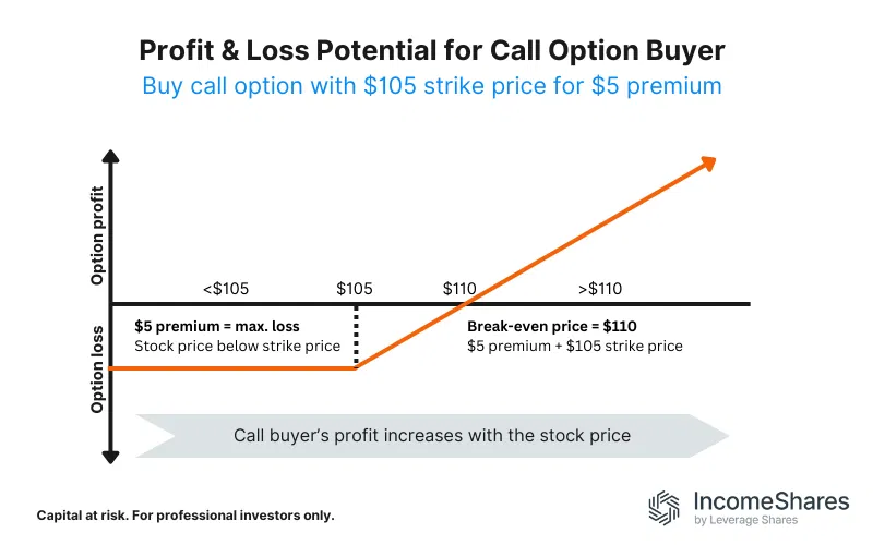
✅ Profit Scenario — Call Option Buyer
A trader buys a call option with the following terms:
| Parameter | Value |
|---|---|
| Strike price | $105 |
| Premium paid | $5 |
| Expiration date | September 20, 2026 |
| Break-even price | $110 |
This call option gives the trader the right (but not the obligation) to buy the underlying stock for $105 on September 20, 2026, no matter how high the stock price goes.
📊 Profit and Loss Outcomes:
–If the stock is below $105 on expiry:
The option expires worthless.
The maximum loss is the premium paid, which is $5.
–If the stock is exactly $110 at expiry:
The option is in the money, but just enough to break even:
(110−105)−5=0
–If the stock is above $110:
The trader earns unlimited upside beyond the break-even price.
2. The Case of a SPX Call Option
Let’s now consider a realistic scenario involving an SPX call option — a European-style, cash-settled derivative contract on the S&P 500 index.
Suppose a trader considers a call option on SPX with the following characteristics:
| Parameter | Value |
|---|---|
| Strike price | 4200 |
| Premium paid | $50 |
| Expiration date | September 20, 2026 |
| Break-even price | 4250 |
This contract gives the buyer the right to receive a cash payout equal to the difference between the SPX index value and the strike price, if the index finishes above 4200 at expiry. Because SPX options are European-style, the option can only be exercised at expiration, and the payout is settled in cash.
This option can be named with different conventions:
Depending on the context (exchange, data provider, or trading platform), the same SPX option can be referred to using various naming conventions. Here are the most common formats:
| Format Type | Example | Description |
|---|---|---|
| Human-readable | SPX-4200C-2026-09-20 | Readable format: underlying, strike, call/put, expiration date |
| OCC Standard Format | SPX260920C04200000 | Used by the Options Clearing Corporation: YYMMDD + C/P + 8-digit strike |
| Bloomberg-style | SPX US 09/20/26 C4200 Index | Used in terminals like Bloomberg |
| Yahoo Finance-style | SPX Sep 20 2026 4200 Call | Often seen on retail platforms and data aggregators |
All of these refer to the same contract: a European-style SPX call option with a strike price of 4200, expiring on September 20, 2026.
3. Develop a SPX US 09/20/26 C4200 European Style Option Pricer
This C++ example uses QuantLib to price a European-style SPX call option by first calculating its implied volatility from a given market price, then re-pricing the option using that implied vol.
It’s a simple, clean way to bridge real-world option data with model-based pricing.
Perfect for understanding how traders extract market expectations from prices.
#include <ql/quantlib.hpp>
#include <iostream>

using namespace QuantLib;

int main() {
    // Set today's date
    Date today(20, June, 2026);
    Settings::instance().evaluationDate() = today;

    // Option parameters
    Real strike = 4200.0;
    Date expiry(20, September, 2026);
    Real marketPrice = 150.0;   // Market price of the call
    Real spot = 4350.0;         // SPX index level
    Rate r = 0.035;             // Risk-free rate
    Volatility volGuess = 0.20; // Initial guess

    // Day count convention
    DayCounter dc = Actual365Fixed();

    // Set up handles
    Handle<Quote> spotH(boost::make_shared<SimpleQuote>(spot));
    Handle<YieldTermStructure> rH(boost::make_shared<FlatForward>(today, r, dc));
    Handle<BlackVolTermStructure> volH(boost::make_shared<BlackConstantVol>(today, TARGET(), volGuess, dc));

    // Build option
    auto payoff = boost::make_shared<PlainVanillaPayoff>(Option::Call, strike);
    auto exercise = boost::make_shared<EuropeanExercise>(expiry);
    EuropeanOption option(payoff, exercise);

    auto process = boost::make_shared<BlackScholesProcess>(spotH, rH, volH);

    // Calculate implied volatility
    Volatility impliedVol = option.impliedVolatility(marketPrice, process);
    std::cout << "Implied Volatility: " << impliedVol * 100 << "%" << std::endl;

    // Re-price using implied vol
    Handle<BlackVolTermStructure> volH_real(boost::make_shared<BlackConstantVol>(today, TARGET(), impliedVol, dc));
    auto process_real = boost::make_shared<BlackScholesProcess>(spotH, rH, volH_real);
    option.setPricingEngine(boost::make_shared<AnalyticEuropeanEngine>(process_real));

    std::cout << "Recalculated Option Price: " << option.NPV() << std::endl;
    return 0;
}
🔍 Explanation of the Steps
- Set market inputs: We define the option’s parameters, spot price, risk-free rate, and the option’s market price.
- Estimate implied volatility: QuantLib inverts the Black-Scholes formula to solve for the volatility that matches the market price.
- Reprice with implied vol: We plug the implied volatility back into the model to confirm the match and prepare for any further analysis (Greeks, charts, etc.).
4. Ideas of Experiments
Once your European style option pricer works for this SPX call option, you can extend it with experiments to better understand option dynamics and sensitivities:
- Vary the Spot Price
Observe how the option value changes as SPX moves from 4000 to 4600. Plot a payoff curve at expiry and at time-to-expiry. - Strike Sweep (Volatility Smile)
Keep the expiry fixed and compute implied volatility across a range of strike prices (e.g., 3800 to 4600). Plot the resulting smile or skew. - Volatility Sensitivity (Vega Analysis)
Change implied volatility from 10% to 50% and plot the change in option price. This shows how much the price depends on volatility. - Time to Expiry (Theta Decay)
Fix all inputs and reduce the time to maturity in steps (e.g., 90 → 60 → 30 → 1 day). Plot how the option price decays over time. - Compare Historical vs Implied Vol
Calculate historical volatility from past SPX prices and compare it to the implied vol from market pricing. Plot both for the same strike/expiry. - Greeks Across Time or Price
Plot delta, gamma, vega as functions of SPX price or time to expiry using QuantLib’soption.delta()etc. - Stress Test Scenarios
Combine spot drops and volatility spikes to simulate market panic — useful to understand hedging behavior.
Each of these can generate powerful charts or tables to enhance your article or future dashboards. Let me know if you’d like example plots or code snippets for any of them.