
Credit Valuation Adjustment (CVA) is the adjustment applied to a derivative’s default-free value to account for this counterparty credit risk. In simple terms, CVA is the present value of the expected loss caused by the possibility that the counterparty defaults while the derivative has positive exposure.
1. Understand the CVA Formula
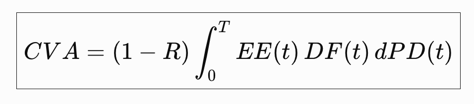
The term CVA (Credit Valuation Adjustment) is defined as:
The discretized version of that integral is a sum:
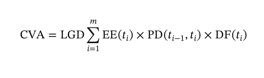
Credit Valuation Adjustment (CVA) Components
- LGD (Loss Given Default): The percentage of exposure lost if the counterparty defaults (1 – Recovery Rate).
- EE (Expected Exposure): The average positive value or market exposure of the portfolio at future time \(t_{i}\).
- PD (Probability of Default): The marginal chance that the counterparty defaults during the specific time interval.
- DF (Discount Factor): The present value factor that discounts future cash flows back to today.
- R (Recovery Rate) is the recovery rate of the counterparty.
A way to explain it is: at every future date, ask how much we could lose, how likely the counterparty is to default during that period, and what that loss is worth today.
Then add everything up.
First divide the life of the portfolio into dates:
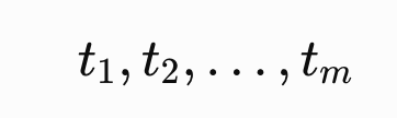
For all of those, it’s possible to calculate the Expected Exposure (EE). If the derivative has positive value, the counterparty owes you money and you are exposed to their default:
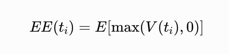
This is often obtained by simulating market variables such as interest rates, FX rates, equity prices, etc.
For example:
| Year | Expected Exposure |
|---|---|
| 1 | £10m |
| 2 | £14m |
| 3 | £9m |
| 4 | £5m |
| 5 | £1m |
Why?
If the counterparty defaults when they owe you nothing, there is essentially no credit loss. CVA therefore depends on the amount you expect to be exposed to at the time of default.
For a real portfolio, this calculation should also reflect things such as netting and collateral.
Next calculate:
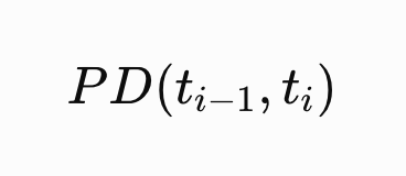
This is the probability that the counterparty survives until ti−1 and then defaults between ti−1 and ti.
For example:
| Period | Incremental PD |
|---|---|
| Year 0–1 | 1.0% |
| Year 1–2 | 1.2% |
| Year 2–3 | 1.4% |
| Year 3–4 | 1.5% |
| Year 4–5 | 1.6% |
An important point is that we use the incremental default probability, not simply the cumulative probability of default by each year.
Why?
Default can only happen once. Each interval represents a different possible default time, so we want the probability that default occurs specifically in that interval.
Now apply LGD (Loss Given Default): if the counterparty defaults, you do not necessarily lose the entire exposure.

For example, if the assumed recovery rate is 40%: LGD=1−0.40=60%
If exposure at default is £10m: Expected loss if default occurs=10m×60%=£6m
Why?
Some money may be recovered through bankruptcy proceedings, collateral, restructuring, etc. CVA should measure the expected economic loss, rather than assuming a 100% loss.
But a loss occurring several years from now is not worth the same amount as a loss today.
So multiply by:
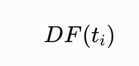
For example, if the 3-year discount factor is 0.92: £1m expected loss in year 3→£0.92m present value
Why?
CVA is a present-value adjustment to the value of the derivative today.
So, for each interval, we can calculate:

And finally sum across all periods:

Which can be summarized as:

Which is very close to the definition of expected loss:

2. How does CVA reduce the value of a derivative?
Credit Valuation Adjustment or CVA is not just a risk metric. It is a pricing adjustment that reflects the possibility that the counterparty may default before paying everything it owes.
Consider the derivative from the bank’s perspective.
If the derivative has a positive mark-to-market value, it is an asset for the bank: the counterparty owes money to the bank. If the counterparty defaults at that point, the bank may recover only part of that amount.
If the derivative has a negative mark-to-market value, the bank owes money to the counterparty instead. From the perspective of unilateral CVA, this does not create a loss from the counterparty’s default. This is why CVA focuses on positive exposure.
Suppose a derivative has a risk-free value of £10 million. If the counterparty were guaranteed never to default, the bank could value the derivative at the full £10 million.
Now suppose the present value of the expected loss caused by possible counterparty default is £300,000. That expected loss is the CVA.
The credit-adjusted value of the derivative becomes:
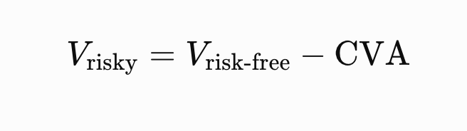
The derivative is worth less because some of its future positive cash flows may never actually be received.
This also explains why two otherwise identical derivatives may have different values when traded with different counterparties. A £10 million receivable from a highly creditworthy counterparty is more valuable than a £10 million receivable from a counterparty with a significant probability of default.
CVA provides a way to incorporate that difference directly into the valuation.
The relationship also gives some useful intuition: PD↑⇒CVA↑⇒Vrisky↓
If the counterparty becomes more likely to default, CVA increases and the derivative becomes less valuable.
Similarly: EE↑⇒CVA↑⇒Vrisky↓
If the bank expects to be owed more money in the future, more value is at risk if the counterparty defaults.
Conversely, better collateralisation, stronger netting agreements or an improvement in the counterparty’s credit quality can reduce expected losses and therefore reduce CVA.
So the key idea is simple:
CVA is the monetary value of counterparty credit risk embedded in the price of the derivative.
3. Implementation in C++
There are several ways to implement a CVA calculation in C++, depending on how much of the pricing stack you want to build yourself.
At the simplest level, you can assume that the expected exposure profile, default probabilities and discount factors have already been calculated. CVA then becomes a straightforward aggregation: CVA=LGDi∑EE(ti)×PD(ti−1,ti)×DF(ti)
This is a good starting point because it isolates the CVA calculation from the more complex problem of generating future exposures.
A more complete implementation would typically involve one of the following approaches:
- Precomputed exposure profiles — read EE, PD and discount curves from upstream systems and aggregate them. This is the simplest approach.
- Monte Carlo simulation — simulate future market states, reprice the portfolio at each future date, and estimate EE(t) from the resulting exposure distribution.
- QuantLib — use existing pricing engines, yield curves, credit curves and stochastic processes rather than implementing every component from scratch.
- Production CVA engine — combine trade pricing, netting sets, collateral agreements, market simulation, credit curves and aggregation across thousands or millions of trades.
For illustration, we can start with the first approach.
Suppose the expected exposure profile is:
Year EE Incremental PD DF
1 10.0m 1.0% 0.97
2 14.0m 1.2% 0.94
3 8.0m 1.4% 0.91
A simple C++ implementation is then:
#include <iostream>
#include <vector>
#include <stdexcept>

struct CVAPoint {
    double expectedExposure;
    double defaultProbability;
    double discountFactor;
};

double calculateCVA(
    const std::vector<CVAPoint>& profile,
    double recoveryRate)
{
    if (recoveryRate < 0.0 || recoveryRate > 1.0) {
        throw std::invalid_argument("Invalid recovery rate");
    }

    const double lgd = 1.0 - recoveryRate;

    double cva = 0.0;

    for (const auto& point : profile) {
        cva += point.expectedExposure
             * point.defaultProbability
             * point.discountFactor
             * lgd;
    }

    return cva;
}

int main()
{
    std::vector<CVAPoint> profile = {
        {10'000'000.0, 0.010, 0.97},
        {14'000'000.0, 0.012, 0.94},
        { 8'000'000.0, 0.014, 0.91}
    };

    const double recoveryRate = 0.40;

    const double cva = calculateCVA(profile, recoveryRate);

    std::cout << "CVA = £" << cva << '\n';
}
For the first year, for example: 10,000,000×0.01×0.97×0.60=58,200
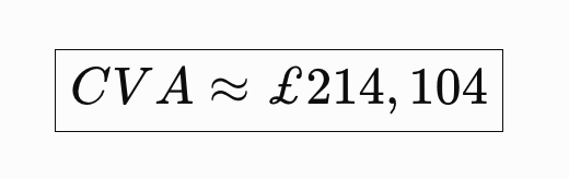
The three contributions are approximately: 58,200+94,752+61,152=214,104
so the resulting CVA is approximately:
4. CVA as part of the XVA framework
CVA is one component of the broader XVA framework used to adjust the clean, or risk-free, value of a derivative for costs and risks that are not captured by the classical pricing model.
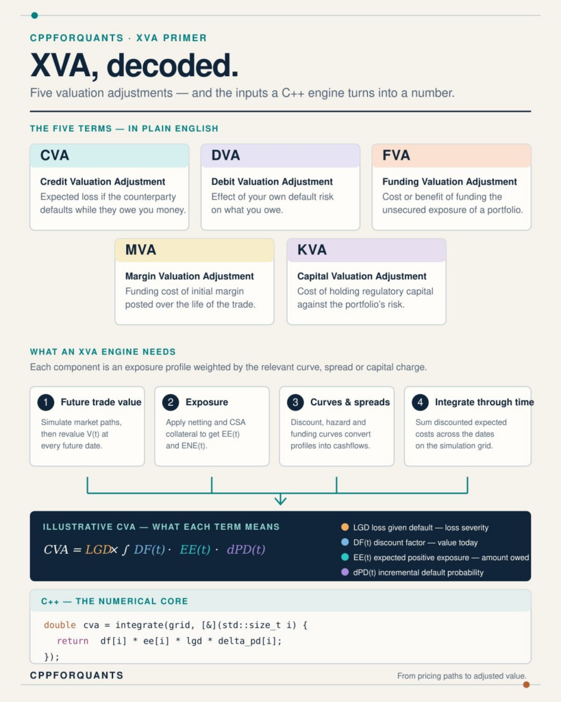
A useful way to think about the XVA stack is:
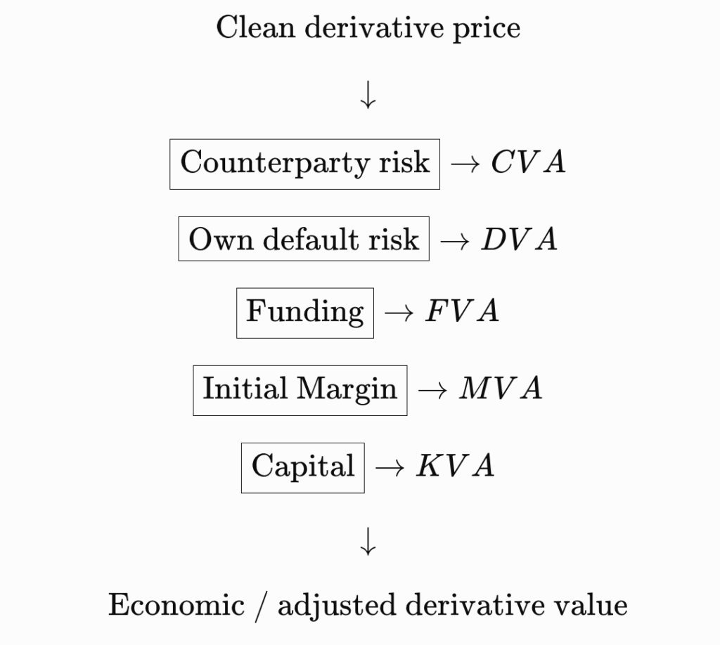
This is why CVA should not be viewed as an isolated calculation. It is one part of a much larger framework used by banks to determine the true economic cost of entering into and maintaining a derivative position.
It also explains why the same exposure simulation infrastructure can often support several XVA calculations. Once a system can simulate future portfolio values, collateral and exposure distributions, those simulations can be reused to calculate CVA, DVA, FVA, MVA and other adjustments.
In practice, this is one of the reasons XVA systems can become computationally demanding: a large bank may need to simulate future market states and reprice millions of trades across thousands of counterparties and many future time steps before the different valuation adjustments can be calculated.
5. 10 interview questions about CVA
1. What is CVA?
CVA is the credit valuation adjustment made to a derivative’s value to account for the possibility that the counterparty defaults.
2. Why does CVA reduce a derivative’s value?
Because a positive future payoff is worth less if there is a chance the counterparty will not fully pay it.
3. What is expected exposure?
Expected exposure is the average amount the bank expects to be owed by the counterparty at a future date.
4. What is the difference between EE and PFE?
EE is the average future exposure, while PFE measures a high percentile of potential exposure and focuses more on tail risk.
5. Where do default probabilities come from?
They are generally derived from the counterparty’s credit curve, often using CDS or bond market information.
6. Why use incremental default probabilities?
Because CVA needs the probability that default occurs within each specific time period, without double-counting default risk.
7. How do netting and collateral affect CVA?
They reduce the amount exposed to counterparty default and therefore generally reduce CVA.
8. What is wrong-way risk?
Wrong-way risk occurs when exposure increases at the same time as the counterparty becomes more likely to default.
9. How is CVA calculated with Monte Carlo simulation?
Future market scenarios are simulated, the portfolio is repriced, exposures are calculated, and the resulting expected losses are aggregated.
10. How does CVA fit into XVA?
CVA is the counterparty-credit component of XVA, alongside adjustments for own credit risk, funding, margin and capital costs.