ClickHouse for Quantitative Finance: Market Data at Scale in C++

58

Quantitative finance produces a lot of data. Market ticks, order books, historical prices, risk scenarios, P&L series, backtest results and model outputs can quickly grow from millions to billions of rows. At that scale, the database starts to matter: ClickHouse is a high-performance columnar database written in C++ and designed for analytical workloads over very large datasets. For all those reasons, ClickHouse for quantitative finance is a good fit.

Instead of optimizing for frequent row-by-row updates, it is built to scan, aggregate and filter huge amounts of data quickly which makes it particularly interesting for quantitative research, market data analysis and risk systems. In this article, we will look at how ClickHouse can be used to store and query financial market data, why its architecture fits many quant workloads, and how a C++ application can interact with it in practice.

1. What is ClickHouse?

ClickHouse is an open-source, column-oriented database designed for analytical workloads. More specifically, it is an OLAP database (Online Analytical Processing) built to scan, filter and aggregate very large datasets quickly.

This is quite different from a traditional transactional database such as PostgreSQL or MySQL.

In a row-oriented database, the values belonging to one record are typically stored together. This works well when an application frequently reads or updates individual rows.

ClickHouse instead stores data by column. If a table contains:

• timestamp
• symbol
• bid
• ask
• volume
• exchange

and a query only needs timestamp, symbol and bid, ClickHouse can largely avoid reading the other columns. This reduces the amount of data that needs to be read and also allows similar values within each column to be compressed efficiently.

This architecture is particularly effective for queries such as:

SELECT
    symbol,
    avg(price)
FROM trades
WHERE timestamp >= now() - INTERVAL 1 DAY
GROUP BY symbol;

Such a query may need to inspect millions or billions of observations but only a small number of columns.

That is exactly the kind of workload that appears frequently in quantitative finance: querying historical prices, aggregating trades, analysing market data, calculating statistics over time windows, or examining large sets of risk and simulation results.

ClickHouse for quantitative finance is therefore not necessarily a replacement for the transactional database behind an application. It is better thought of as a high-performance analytical engine for datasets where fast reads, filtering and aggregation at scale matter more than frequent row-by-row updates.

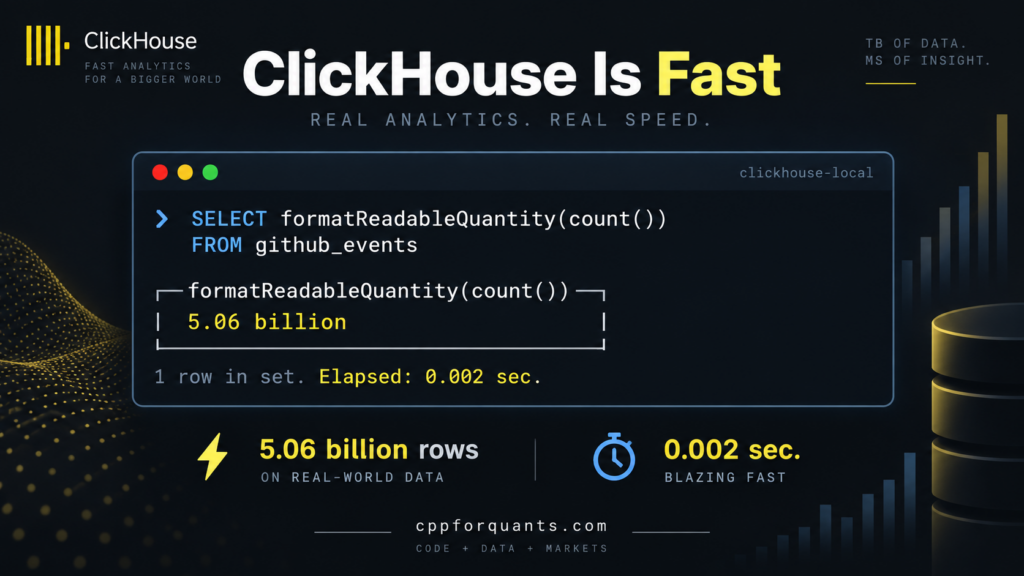
How fast? Very fast.

2.Why columnar databases fit quantitative finance

Quantitative finance is naturally data-intensive. A market data table may contain billions of observations across prices, volumes, instruments, venues and timestamps. Risk systems can generate similarly large datasets from Monte Carlo scenarios, sensitivities, exposures and P&L calculations.

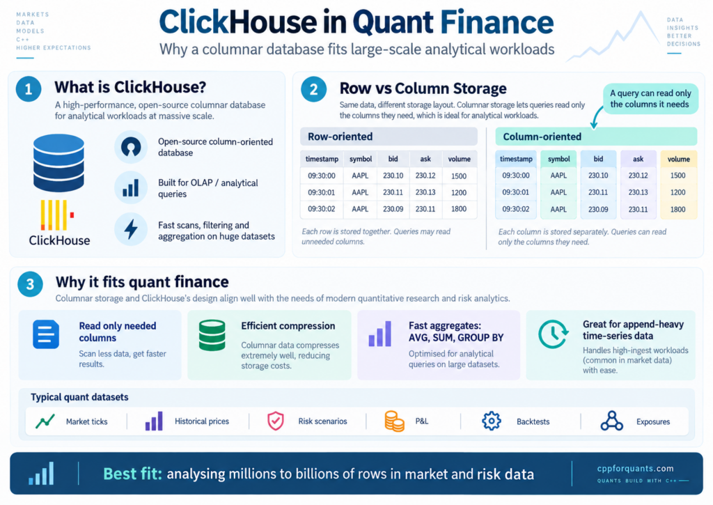
The important point is that quants rarely need every field for every observation.

Consider a table containing:

timestamp
symbol
bid
ask
volume
exchange
currency

A query calculating the average spread for a given instrument may only need timestamp, bid and ask. A row-oriented database typically stores all the values belonging to each observation together. A columnar database stores values from the same column together instead.

Conceptually:

Row-oriented

09:30:00 | AAPL | 230.10 | 230.12 | 1500 | NASDAQ
09:30:01 | AAPL | 230.11 | 230.13 | 1200 | NASDAQ
09:30:02 | AAPL | 230.09 | 230.11 | 1800 | NASDAQ

versus:

Column-oriented

timestamp: 09:30:00, 09:30:01, 09:30:02, ...
symbol:    AAPL, AAPL, AAPL, ...
bid:       230.10, 230.11, 230.09, ...
ask:       230.12, 230.13, 230.11, ...
volume:    1500, 1200, 1800, ...

This has several advantages for quantitative workloads.

Reading only what is needed

Many financial queries operate on a subset of the available variables. If we want to calculate the average bid-ask spread:

SELECT avg(ask - bid)
FROM market_data
WHERE symbol = 'AAPL';

the database mainly needs the symbol, bid and ask columns.

With billions of rows, avoiding unnecessary columns can significantly reduce the amount of data that must be read from storage.

Efficient compression

Financial datasets also contain a lot of repeated or highly structured information.

A symbol column may contain the same ticker millions of times. Exchange and currency fields have low cardinality. Timestamps are ordered and numerical values often change gradually.

Storing similar values together makes this data highly compressible. Better compression means less disk space, but more importantly it can mean less data to read from disk when executing analytical queries.

Fast aggregation

Quantitative analysis frequently involves operations such as:

AVG
SUM
MIN
MAX
COUNT
quantiles
GROUP BY

For example:

SELECT
    symbol,
    avg(price),
    max(price),
    min(price)
FROM trades
WHERE timestamp >= '2026-01-01'
GROUP BY symbol;

Instead of retrieving individual transactions one at a time, the objective is to process a very large number of observations and derive statistics from them.

That is exactly the workload column-oriented databases are designed to handle.

A natural match for time-series market data

Market data is also usually append-heavy: that’s why Clickhouse for quantitative finance is interesting.

New ticks arrive continuously:

t1 → price
t2 → price
t3 → price
...
tn → price

Historical observations are then queried repeatedly for research, backtesting, monitoring and analysis.

This pattern — large volumes of data being appended and subsequently scanned or aggregated — fits ClickHouse particularly well.

The same idea applies beyond market ticks. A quant platform might use a columnar database to analyse:

• historical prices and trades,
• order-book observations,
• Greeks and sensitivities,
• P&L histories,
• backtest results,
• Monte Carlo scenarios,
• counterparty exposures,
• model predictions,
• risk metrics.

This does not mean every financial database should be columnar. Transactional systems still need databases optimized for individual inserts, updates and lookups.

But when the problem becomes “analyse hundreds of millions or billions of observations quickly”, the columnar model becomes particularly attractive — and this is the type of problem ClickHouse was built to solve.

3. Accessing ClickHouse from C++

For a C++ quant application, ClickHouse can be accessed using the official clickhouse-cpp client library.

The client is written in C++17 and communicates with ClickHouse through its native binary protocol. It provides direct support for executing SQL queries and sending or receiving data in ClickHouse’s native columnar Block format.

A minimal connection looks like this:

#include <clickhouse/client.h>

using namespace clickhouse;

int main()
{
    Client client(ClientOptions()
        .SetHost("localhost")
        .SetPort(9000));

    client.Execute("SELECT 1");
}

The interesting part for quantitative applications is that the C++ API is also column-oriented.

Imagine that we want to store some market data:

CREATE TABLE market_data
(
    timestamp DateTime64(3),
    symbol String,
    bid Float64,
    ask Float64,
    volume UInt64
)
ENGINE = MergeTree
ORDER BY (symbol, timestamp);

We can construct the corresponding columns directly in C++:

#include <clickhouse/client.h>

using namespace clickhouse;

int main()
{
    Client client(ClientOptions().SetHost("localhost"));

    auto symbol = std::make_shared<ColumnString>();
    auto bid    = std::make_shared<ColumnFloat64>();
    auto ask    = std::make_shared<ColumnFloat64>();
    auto volume = std::make_shared<ColumnUInt64>();

    symbol->Append("AAPL");
    symbol->Append("AAPL");
    symbol->Append("MSFT");

    bid->Append(230.10);
    bid->Append(230.11);
    bid->Append(415.20);

    ask->Append(230.12);
    ask->Append(230.13);
    ask->Append(415.24);

    volume->Append(1500);
    volume->Append(1200);
    volume->Append(900);

    Block block;

    block.AppendColumn("symbol", symbol);
    block.AppendColumn("bid", bid);
    block.AppendColumn("ask", ask);
    block.AppendColumn("volume", volume);

    client.Insert("market_data", block);
}

Instead of inserting one trade or tick at a time, we construct a batch of columns and send the entire block to ClickHouse.

This is a natural model for market data pipelines:

Market feed
    ↓
C++ application
    ↓
Accumulate ticks in memory
    ↓
Build ClickHouse Block
    ↓
Batch insert
    ↓
ClickHouse

For large datasets, clickhouse-cpp also supports a streaming batch pattern using BeginInsert, SendInsertBlock and EndInsert, allowing applications to send multiple blocks without keeping the entire dataset in memory.

Querying market data

Reading data follows the same idea. Query results are returned as blocks containing typed columns.

For example:

client.Select(
    R"(
        SELECT
            symbol,
            avg(ask - bid) AS avg_spread
        FROM market_data
        GROUP BY symbol
    )",
    [](const Block& block)
    {
        auto symbol =
            block[0]->As<ColumnString>();

        auto spread =
            block[1]->As<ColumnFloat64>();

        for (size_t i = 0; i < block.GetRowCount(); ++i)
        {
            std::cout
                << symbol->At(i)
                << " "
                << spread->At(i)
                << '\n';
        }
    });

The SQL computation happens inside ClickHouse, while the C++ application receives only the aggregated result.

This distinction is important.

Rather than loading hundreds of millions of market observations into C++ and calculating statistics locally, we can push filtering and aggregation to ClickHouse:

Bad approach

ClickHouse
   ↓
500 million rows
   ↓
C++
   ↓
Calculate statistics


Better approach

ClickHouse
   ↓
Filter + aggregate
   ↓
Small result
   ↓
C++

For a quant system, C++ can therefore remain responsible for pricing, simulation or trading logic, while ClickHouse handles the large analytical dataset behind it.

This combination is particularly attractive when an application needs to process large volumes of market data without turning the C++ process itself into a database engine.

4. An Example of Low-Latency Architecture with ClickHouse

ClickHouse can fit very well into a low-latency trading or market-data architecture, but usually not in the critical execution path.

A trading system may need to react to market data in microseconds or milliseconds. That part is typically handled in memory, inside C++ processes optimized for deterministic latency.

ClickHouse for quantitative finance instead sits next to the trading system as a fast analytical store.

A simplified architecture could look like this:

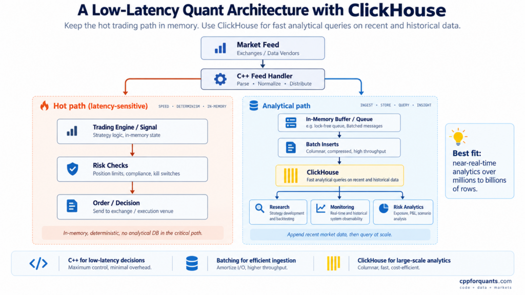
The key idea is to separate the hot path from the analytical path.

The hot path

The hot path contains everything that directly affects a trading decision:

Market data
    ↓
C++ feed handler
    ↓
Pricing / signal
    ↓
Risk checks
    ↓
Order

This path should avoid unnecessary network calls, disk access and database queries.

For the most latency-sensitive systems, the relevant state is usually held directly in memory.

The analytical path

At the same time, the same market data can be copied into an in-memory buffer or message queue:

Market data
    ↓
Buffer
    ↓
Batch
    ↓
ClickHouse

The C++ application may accumulate several thousand observations and periodically send them to ClickHouse as a batch.

ClickHouse can then be used for queries such as:

SELECT
    symbol,
    avg(ask - bid) AS avg_spread,
    sum(volume) AS total_volume
FROM market_data
WHERE timestamp >= now() - INTERVAL 5 MINUTE
GROUP BY symbol;

This gives researchers, monitoring systems and risk processes access to very recent data without adding latency to the trading engine itself.

Why batching matters

A common mistake would be to insert every market tick individually:

Tick
 ↓
INSERT
 ↓
Tick
 ↓
INSERT

That creates unnecessary network and database overhead.

A better approach is:

Tick
Tick
Tick
Tick
...
   ↓
In-memory batch
   ↓
Single ClickHouse insert

For example, a C++ process could buffer 10,000 observations before sending them as one block.

This preserves low latency in the producer while allowing ClickHouse to ingest data efficiently.

A typical division of responsibilities

In such an architecture:

Component	Responsibility
C++	Market-data processing, pricing, signals, execution
Memory / queue	Decoupling the trading path from persistence
ClickHouse	Historical storage and analytical queries
Python / C++ / dashboards	Research, monitoring and risk analytics

This separation is important.

ClickHouse is not replacing the low-latency C++ engine. Instead, it provides a high-performance analytical layer around it.

For quantitative systems, this can be a very effective combination:

C++ for decisions in microseconds or milliseconds, ClickHouse for analysing millions or billions of observations shortly afterwards.

5. Conclusion on Clickhouse

So, how to conclude? Maybe with a comparison with other databases and a list of strengths/weaknesses.

Different systems are optimized for different workloads. PostgreSQL is a strong general-purpose relational database, DuckDB is excellent for local analytical work, kdb+ has a long history in high-performance market data, and InfluxDB is designed around time-series workloads.

ClickHouse sits in a different part of the spectrum. Its main strength is large-scale analytical processing: scanning, filtering and aggregating very large datasets quickly.

The comparison below is therefore not about choosing a universal winner, but about understanding where ClickHouse fits relative to other common database choices in quantitative systems.

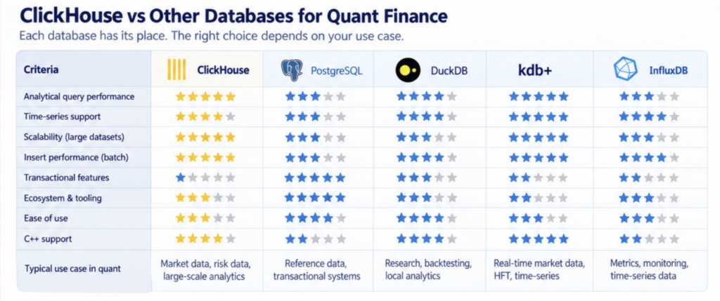
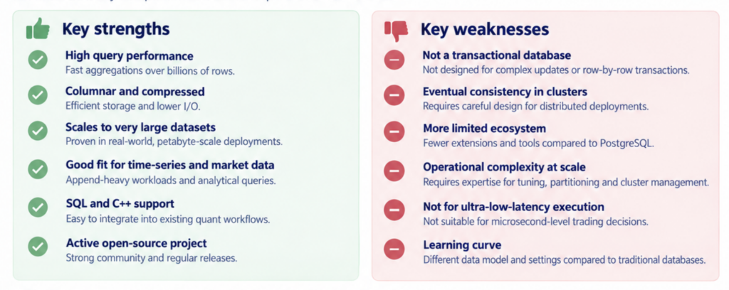
The summary below highlights the main strengths and weaknesses of ClickHouse and helps place it in the broader context of quantitative finance infrastructure: