C++ for Quants
  • Home
  • Contact
  • About
Category:

Performance

montecarlo C++
LibrariesPerformance

Monte Carlo Simulation in C++26 with std::philox_engine

by cppforquants September 12, 2026

Monte Carlo simulation is one of the core tools of quantitative finance. It is used to price derivatives, estimate future exposures, generate market scenarios, and model problems that are difficult to solve analytically. What role plays std::philox_engine in this story?

At the heart of every Monte Carlo simulation is a random number generator. In C++26, the standard library introduces std::philox_engine, a counter-based random number engine designed with large-scale and parallel simulation in mind.A good place to start is the documentation of the library.

In this article, we look at what Philox is, why it is interesting for quantitative finance, and how to use it in a simple Monte Carlo option pricing example. We simulate one million possible terminal stock prices, calculate the payoff of a European call option under each scenario, and estimate the option price from the average discounted payoff.

The goal is not to build a production-grade pricing engine, but to show how a new C++26 feature can fit naturally into a familiar quantitative finance workflow.

1. What Is std::philox_engine?

std::philox_engine is a counter-based pseudo-random number generator introduced in C++26 as part of the <random> library. Unlike traditional generators such as std::mt19937, which evolve a relatively large internal state from one random number to the next, Philox generates values from a combination of a counter and a key. This difference is particularly useful in quantitative finance because counter-based generators are naturally suited to large-scale Monte Carlo simulations:
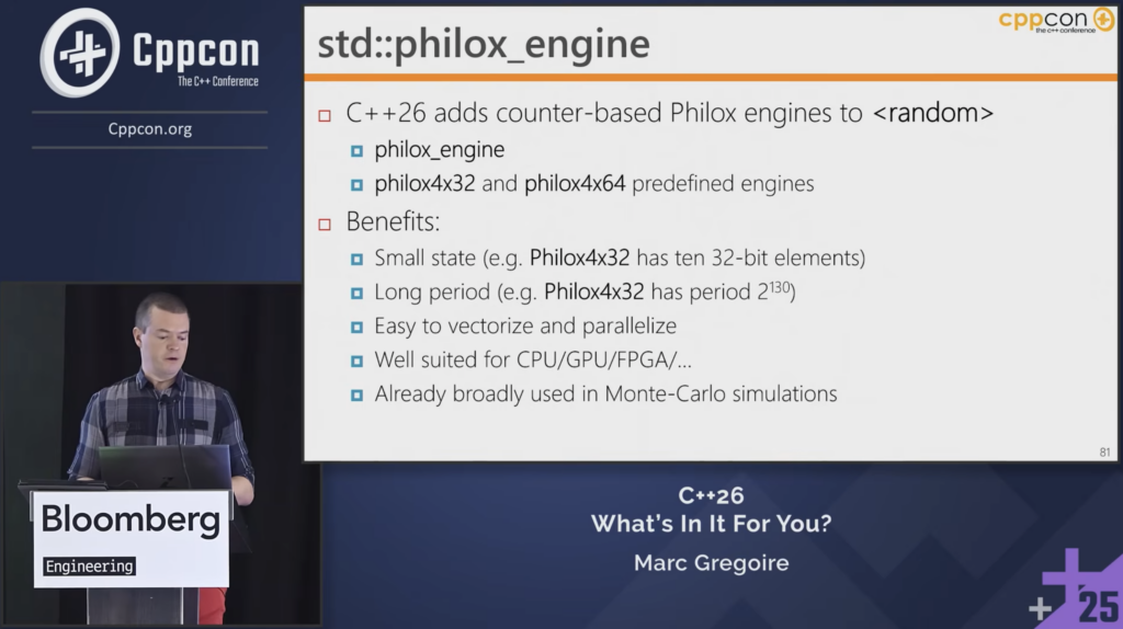
See the full video here:

Conceptually, the generator works like this:

counter + key
     ↓
 Philox rounds
     ↓
pseudo-random values

Instead of relying entirely on a long sequence of state transitions, Philox transforms a counter through several deterministic mixing rounds. Incrementing the counter produces the next block of pseudo-random numbers.

C++26 provides two predefined Philox engines:

std::philox4x32
std::philox4x64

The first generates blocks based on four 32-bit words, while the second uses four 64-bit words. Both predefined versions use 10 Philox rounds.

For example:

#include <iostream>
#include <random>

int main()
{
    std::philox4x32 rng{42};

    std::cout << rng() << '\n';
    std::cout << rng() << '\n';
    std::cout << rng() << '\n';
}

Here, 42 is used to seed the engine. Each call to rng() returns the next pseudo-random integer from the Philox sequence.

The main advantage of Philox is not simply that it generates random numbers. Its design makes independent parts of the random-number space much easier to access and distribute across different computations.

This makes it especially attractive for workloads such as:

  • Monte Carlo option pricing
  • exposure simulation
  • Value at Risk calculations
  • scenario generation
  • multi-threaded simulations
  • GPU-based quantitative workloads

The C++ standard library specifically describes Philox as suitable for Monte Carlo workloads requiring massively parallel random-number generation, and notes that its design is easy to vectorize and parallelize.

Another important property is reproducibility. Given the same seed and the same counter state, Philox produces the same sequence of pseudo-random values. This is extremely useful when debugging or reproducing quantitative simulations.

It is important, however, to distinguish pseudo-randomness from cryptographic randomness. std::philox_engine is designed for numerical simulation and is not a cryptographically secure random-number generator.

For quantitative developers, the key idea is therefore:

Philox is a random-number engine designed around counters rather than a large sequential state, making it particularly well suited to reproducible and highly parallel Monte Carlo simulation.

2. A Simple Monte Carlo Option Pricing Example

To see std::philox_engine in a quantitative finance context, we can use it to price a simple European call option with Monte Carlo simulation.

Assume:

  • spot price (S_0 = 100)
  • strike (K = 100)
  • risk-free rate (r = 5%)
  • volatility (\sigma = 20%)
  • maturity (T = 1) year
  • N simulated paths (e.g: 1,000,000)

Under the Black–Scholes model, the terminal stock price can be simulated as:
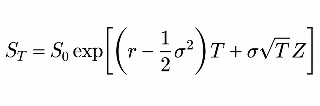
For each simulated terminal stock price STS_T, the payoff of a European call option is:

where KK is the strike price.

After simulating NN paths, we estimate the expected payoff by averaging across all simulations:
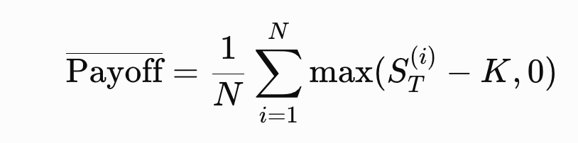
Finally, we discount the expected payoff back to today:
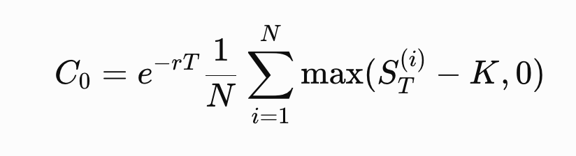
where C0C_0 is the estimated option price, rr is the risk-free rate, and TT is the time to maturity.

3. A C++ Implementation Using std::philox_engine?

Here is a suggestion of implementation:

#include <algorithm>
#include <cmath>
#include <iostream>
#include <random>

int main()
{
    constexpr int paths = 1'000'000;

    const double S0 = 100.0;
    const double K = 100.0;
    const double r = 0.05;
    const double sigma = 0.20;
    const double T = 1.0;

    std::philox4x32 rng{42};
    std::normal_distribution<double> normal(0.0, 1.0);

    double payoff_sum = 0.0;

    for (int i = 0; i < paths; ++i)
    {
        const double z = normal(rng);

        const double ST =
            S0 * std::exp(
                (r - 0.5 * sigma * sigma) * T +
                sigma * std::sqrt(T) * z
            );

        payoff_sum += std::max(ST - K, 0.0);
    }

    const double price =
        std::exp(-r * T) *
        payoff_sum / paths;

    std::cout << "Option price: "
              << price << '\n';
}

Here we create the C++26 predefined 32-bit Philox engine and seed it with 42. std::philox4x32 is one of the predefined specializations of std::philox_engine.

We then combine the engine with:

std::normal_distribution<double> normal(0.0, 1.0);

std::normal_distribution transforms the pseudo-random numbers produced by the engine into normally distributed values with mean (0) and standard deviation (1).

Each call to:

const double z = normal(rng);

therefore gives us one random shock (Z), which we use to generate one possible stock price at maturity.

3. Install C++26, Compile and Execute

If you didn’t install a C++26 compiler yet: it’s the moment! With macOS, a simple brew install will do:

➜ brew install gcc

Then, run a quick check:

➜  g++-16 --version
                                             
g++-16 (Homebrew GCC 16.2.0) 16.2.0
Copyright (C) 2026 Free Software Foundation, Inc.
This is free software; see the source for copying conditions.  There is NO
warranty; not even for MERCHANTABILITY or FITNESS FOR A PARTICULAR PURPOSE.


Yes, you can now compile C++26 code.

Once done, put our implementation above in a montecarlo.cpp, and run:

g++-16 -std=c++26 -O3 -Wall -Wextra montecarlo.cpp -o montecarlo


Then run the binary:

➜  ./montecarlo 
                                                   
Option price: 10.4644

So, what did we just do? A visual summary:

Once the Monte Carlo simulation has produced an average payoff at maturity, that value still represents money received in the future rather than money today. To convert it into a present fair value, we discount it using the risk-free rate which is the exponential term applied to the average payoff.

The key intuition is:

So going the other way:

where rr is the continuously compounded risk-free interest rate and TT is the time to maturity, expressed in years.

4. Why choosing std::philox_engine
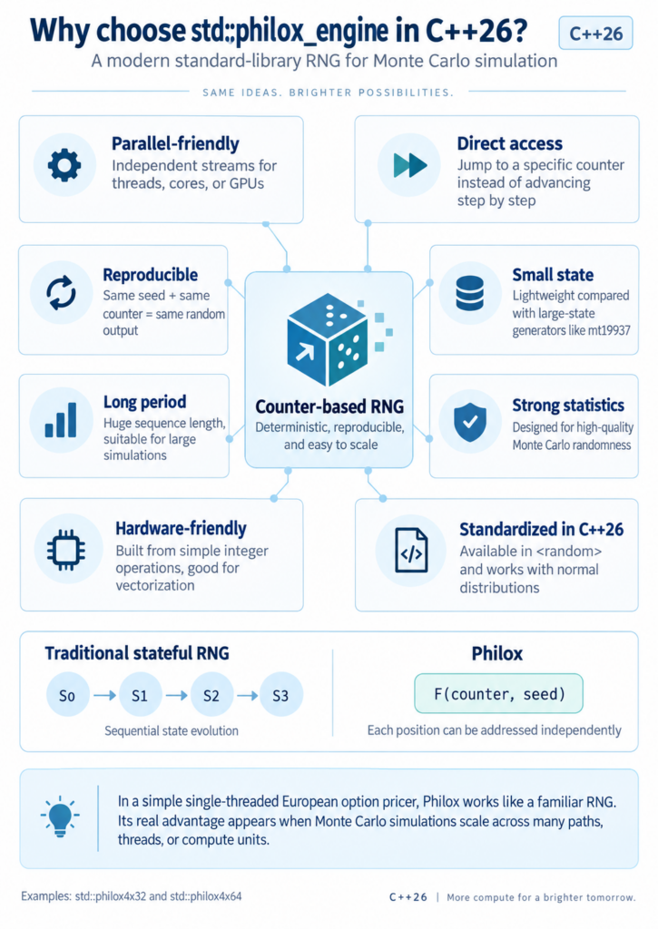
std::philox_engine is an interesting addition to C++26 because it brings a modern counter-based random number generator directly into the standard library. Unlike traditional stateful generators, Philox derives its output from a counter and key, making different regions of the random sequence easy to address independently. This makes the design particularly suitable for large Monte Carlo workloads, where simulations can eventually be split across CPU threads, vector units or GPUs without requiring a single shared random-number-generator state.

std::philox_engine also combines a small internal state, a very long period, strong statistical properties and hardware-friendly integer operations. C++26 additionally exposes set_counter(), allowing an application to position the generator at a specific counter rather than sequentially advancing through the random stream. This is useful for constructing deterministic independent streams and for reproducing individual simulation paths.

Another advantage of standardization is interoperability. std::philox4x32 and std::philox4x64 behave like other C++ random-number engines and can therefore be passed directly to existing facilities such as std::normal_distribution. A Monte Carlo implementation can adopt Philox without redesigning the rest of its simulation pipeline.

In our European option example we use Philox single-threaded, so these parallelism benefits are not yet being exploited. The purpose is to introduce the C++26 engine in the simplest possible setting while using an RNG design that naturally scales toward much larger parallel Monte Carlo simulations.

September 12, 2026 0 comments
Clickhouse for Quantitative Finance
DatabasesPerformance

ClickHouse for Quantitative Finance: Market Data at Scale in C++

by cppforquants September 6, 2026

Quantitative finance produces a lot of data. Market ticks, order books, historical prices, risk scenarios, P&L series, backtest results and model outputs can quickly grow from millions to billions of rows. At that scale, the database starts to matter: ClickHouse is a high-performance columnar database written in C++ and designed for analytical workloads over very large datasets. For all those reasons, ClickHouse for quantitative finance is a good fit.

Instead of optimizing for frequent row-by-row updates, it is built to scan, aggregate and filter huge amounts of data quickly which makes it particularly interesting for quantitative research, market data analysis and risk systems. In this article, we will look at how ClickHouse can be used to store and query financial market data, why its architecture fits many quant workloads, and how a C++ application can interact with it in practice.

1. What is ClickHouse?

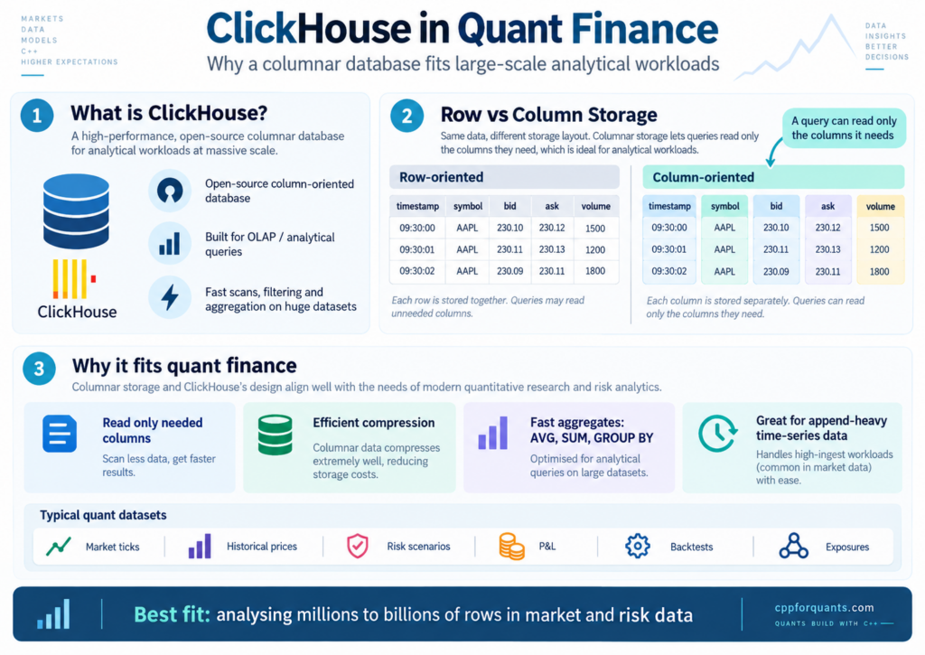
ClickHouse is an open-source, column-oriented database designed for analytical workloads. More specifically, it is an OLAP database (Online Analytical Processing) built to scan, filter and aggregate very large datasets quickly.

This is quite different from a traditional transactional database such as PostgreSQL or MySQL.

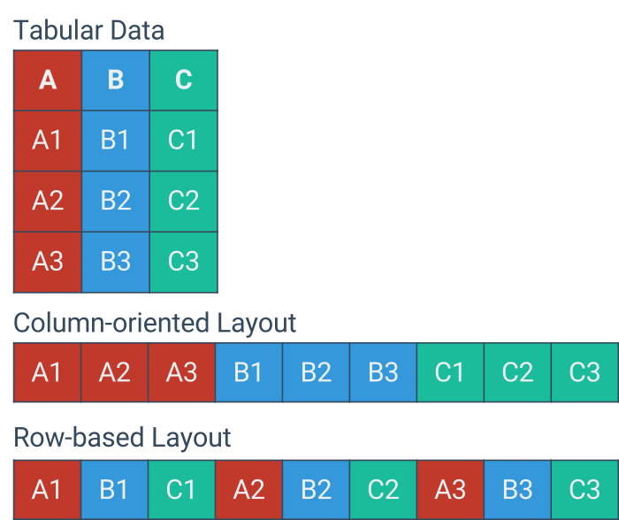
In a row-oriented database, the values belonging to one record are typically stored together. This works well when an application frequently reads or updates individual rows.

ClickHouse instead stores data by column. If a table contains:

  • timestamp
  • symbol
  • bid
  • ask
  • volume
  • exchange

and a query only needs timestamp, symbol and bid, ClickHouse can largely avoid reading the other columns. This reduces the amount of data that needs to be read and also allows similar values within each column to be compressed efficiently.

This architecture is particularly effective for queries such as:

SELECT
    symbol,
    avg(price)
FROM trades
WHERE timestamp >= now() - INTERVAL 1 DAY
GROUP BY symbol;

Such a query may need to inspect millions or billions of observations but only a small number of columns.

That is exactly the kind of workload that appears frequently in quantitative finance: querying historical prices, aggregating trades, analysing market data, calculating statistics over time windows, or examining large sets of risk and simulation results.

ClickHouse for quantitative finance is therefore not necessarily a replacement for the transactional database behind an application. It is better thought of as a high-performance analytical engine for datasets where fast reads, filtering and aggregation at scale matter more than frequent row-by-row updates.

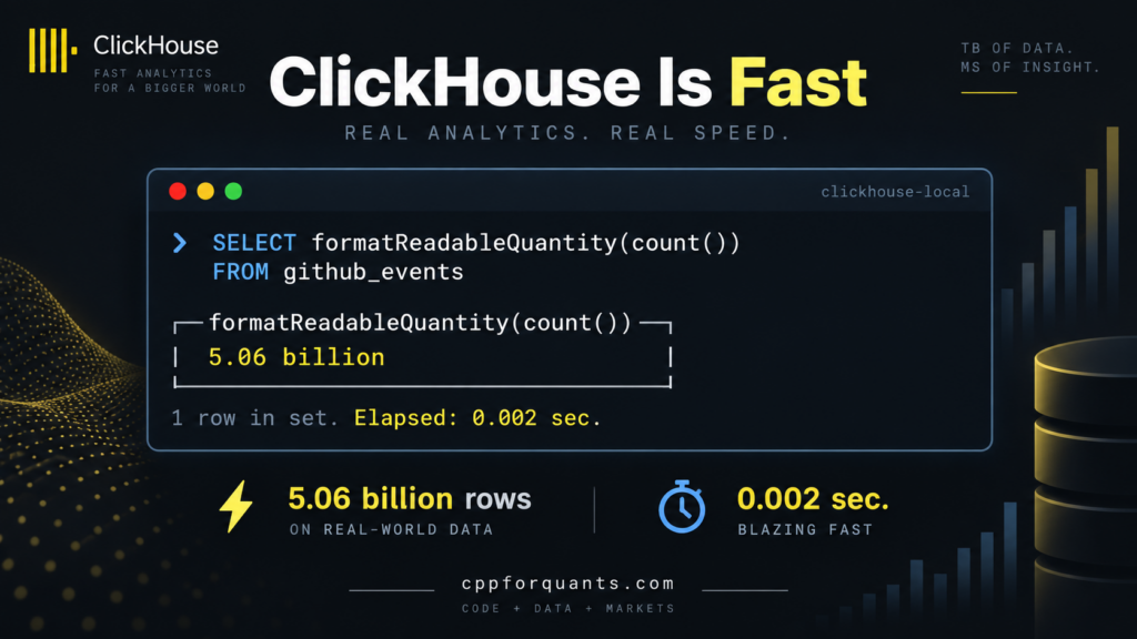
How fast? Very fast.

2.Why columnar databases fit quantitative finance

Quantitative finance is naturally data-intensive. A market data table may contain billions of observations across prices, volumes, instruments, venues and timestamps. Risk systems can generate similarly large datasets from Monte Carlo scenarios, sensitivities, exposures and P&L calculations.

The important point is that quants rarely need every field for every observation.

Consider a table containing:

timestamp
symbol
bid
ask
volume
exchange
currency

A query calculating the average spread for a given instrument may only need timestamp, bid and ask. A row-oriented database typically stores all the values belonging to each observation together. A columnar database stores values from the same column together instead.

Conceptually:

Row-oriented

09:30:00 | AAPL | 230.10 | 230.12 | 1500 | NASDAQ
09:30:01 | AAPL | 230.11 | 230.13 | 1200 | NASDAQ
09:30:02 | AAPL | 230.09 | 230.11 | 1800 | NASDAQ

versus:

Column-oriented

timestamp: 09:30:00, 09:30:01, 09:30:02, ...
symbol:    AAPL, AAPL, AAPL, ...
bid:       230.10, 230.11, 230.09, ...
ask:       230.12, 230.13, 230.11, ...
volume:    1500, 1200, 1800, ...

This has several advantages for quantitative workloads.

Reading only what is needed

Many financial queries operate on a subset of the available variables. If we want to calculate the average bid-ask spread:

SELECT avg(ask - bid)
FROM market_data
WHERE symbol = 'AAPL';

the database mainly needs the symbol, bid and ask columns.

With billions of rows, avoiding unnecessary columns can significantly reduce the amount of data that must be read from storage.

Efficient compression

Financial datasets also contain a lot of repeated or highly structured information.

A symbol column may contain the same ticker millions of times. Exchange and currency fields have low cardinality. Timestamps are ordered and numerical values often change gradually.

Storing similar values together makes this data highly compressible. Better compression means less disk space, but more importantly it can mean less data to read from disk when executing analytical queries.

Fast aggregation

Quantitative analysis frequently involves operations such as:

AVG
SUM
MIN
MAX
COUNT
quantiles
GROUP BY

For example:

SELECT
    symbol,
    avg(price),
    max(price),
    min(price)
FROM trades
WHERE timestamp >= '2026-01-01'
GROUP BY symbol;

Instead of retrieving individual transactions one at a time, the objective is to process a very large number of observations and derive statistics from them.

That is exactly the workload column-oriented databases are designed to handle.

A natural match for time-series market data

Market data is also usually append-heavy: that’s why Clickhouse for quantitative finance is interesting.

New ticks arrive continuously:

t1 → price
t2 → price
t3 → price
...
tn → price

Historical observations are then queried repeatedly for research, backtesting, monitoring and analysis.

This pattern — large volumes of data being appended and subsequently scanned or aggregated — fits ClickHouse particularly well.

The same idea applies beyond market ticks. A quant platform might use a columnar database to analyse:

  • historical prices and trades,
  • order-book observations,
  • Greeks and sensitivities,
  • P&L histories,
  • backtest results,
  • Monte Carlo scenarios,
  • counterparty exposures,
  • model predictions,
  • risk metrics.

This does not mean every financial database should be columnar. Transactional systems still need databases optimized for individual inserts, updates and lookups.

But when the problem becomes “analyse hundreds of millions or billions of observations quickly”, the columnar model becomes particularly attractive — and this is the type of problem ClickHouse was built to solve.

3. Accessing ClickHouse from C++

For a C++ quant application, ClickHouse can be accessed using the official clickhouse-cpp client library.

The client is written in C++17 and communicates with ClickHouse through its native binary protocol. It provides direct support for executing SQL queries and sending or receiving data in ClickHouse’s native columnar Block format.

A minimal connection looks like this:

#include <clickhouse/client.h>

using namespace clickhouse;

int main()
{
    Client client(ClientOptions()
        .SetHost("localhost")
        .SetPort(9000));

    client.Execute("SELECT 1");
}

The interesting part for quantitative applications is that the C++ API is also column-oriented.

Imagine that we want to store some market data:

CREATE TABLE market_data
(
    timestamp DateTime64(3),
    symbol String,
    bid Float64,
    ask Float64,
    volume UInt64
)
ENGINE = MergeTree
ORDER BY (symbol, timestamp);

We can construct the corresponding columns directly in C++:

#include <clickhouse/client.h>

using namespace clickhouse;

int main()
{
    Client client(ClientOptions().SetHost("localhost"));

    auto symbol = std::make_shared<ColumnString>();
    auto bid    = std::make_shared<ColumnFloat64>();
    auto ask    = std::make_shared<ColumnFloat64>();
    auto volume = std::make_shared<ColumnUInt64>();

    symbol->Append("AAPL");
    symbol->Append("AAPL");
    symbol->Append("MSFT");

    bid->Append(230.10);
    bid->Append(230.11);
    bid->Append(415.20);

    ask->Append(230.12);
    ask->Append(230.13);
    ask->Append(415.24);

    volume->Append(1500);
    volume->Append(1200);
    volume->Append(900);

    Block block;

    block.AppendColumn("symbol", symbol);
    block.AppendColumn("bid", bid);
    block.AppendColumn("ask", ask);
    block.AppendColumn("volume", volume);

    client.Insert("market_data", block);
}

Instead of inserting one trade or tick at a time, we construct a batch of columns and send the entire block to ClickHouse.

This is a natural model for market data pipelines:

Market feed
    ↓
C++ application
    ↓
Accumulate ticks in memory
    ↓
Build ClickHouse Block
    ↓
Batch insert
    ↓
ClickHouse

For large datasets, clickhouse-cpp also supports a streaming batch pattern using BeginInsert, SendInsertBlock and EndInsert, allowing applications to send multiple blocks without keeping the entire dataset in memory.

Querying market data

Reading data follows the same idea. Query results are returned as blocks containing typed columns.

For example:

client.Select(
    R"(
        SELECT
            symbol,
            avg(ask - bid) AS avg_spread
        FROM market_data
        GROUP BY symbol
    )",
    [](const Block& block)
    {
        auto symbol =
            block[0]->As<ColumnString>();

        auto spread =
            block[1]->As<ColumnFloat64>();

        for (size_t i = 0; i < block.GetRowCount(); ++i)
        {
            std::cout
                << symbol->At(i)
                << " "
                << spread->At(i)
                << '\n';
        }
    });

The SQL computation happens inside ClickHouse, while the C++ application receives only the aggregated result.

This distinction is important.

Rather than loading hundreds of millions of market observations into C++ and calculating statistics locally, we can push filtering and aggregation to ClickHouse:

Bad approach

ClickHouse
   ↓
500 million rows
   ↓
C++
   ↓
Calculate statistics


Better approach

ClickHouse
   ↓
Filter + aggregate
   ↓
Small result
   ↓
C++

For a quant system, C++ can therefore remain responsible for pricing, simulation or trading logic, while ClickHouse handles the large analytical dataset behind it.

This combination is particularly attractive when an application needs to process large volumes of market data without turning the C++ process itself into a database engine.


4. An Example of Low-Latency Architecture with ClickHouse

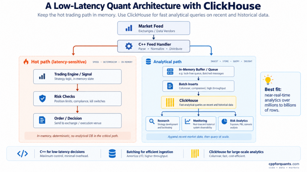
ClickHouse can fit very well into a low-latency trading or market-data architecture, but usually not in the critical execution path.

A trading system may need to react to market data in microseconds or milliseconds. That part is typically handled in memory, inside C++ processes optimized for deterministic latency.

ClickHouse for quantitative finance instead sits next to the trading system as a fast analytical store.

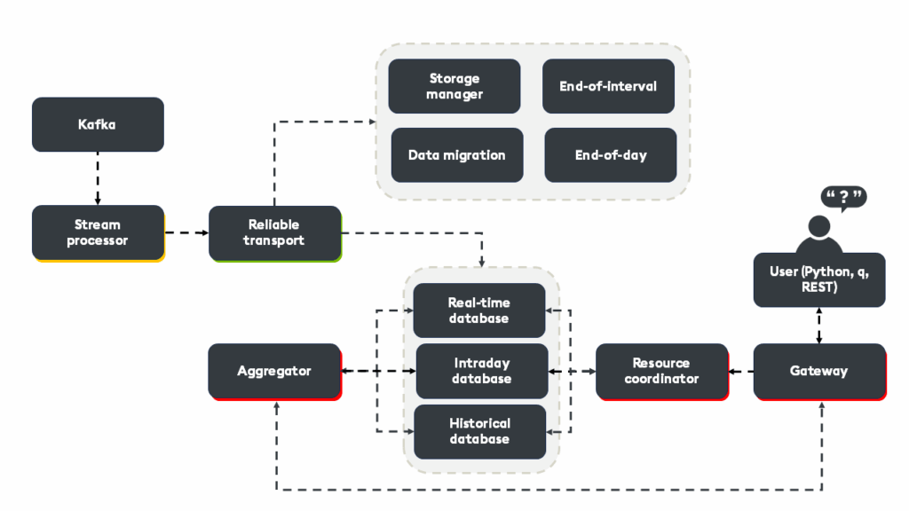
A simplified architecture could look like this:


The key idea is to separate the hot path from the analytical path.

The hot path

The hot path contains everything that directly affects a trading decision:

Market data
    ↓
C++ feed handler
    ↓
Pricing / signal
    ↓
Risk checks
    ↓
Order

This path should avoid unnecessary network calls, disk access and database queries.

For the most latency-sensitive systems, the relevant state is usually held directly in memory.

The analytical path

At the same time, the same market data can be copied into an in-memory buffer or message queue:

Market data
    ↓
Buffer
    ↓
Batch
    ↓
ClickHouse

The C++ application may accumulate several thousand observations and periodically send them to ClickHouse as a batch.

ClickHouse can then be used for queries such as:

SELECT
    symbol,
    avg(ask - bid) AS avg_spread,
    sum(volume) AS total_volume
FROM market_data
WHERE timestamp >= now() - INTERVAL 5 MINUTE
GROUP BY symbol;

This gives researchers, monitoring systems and risk processes access to very recent data without adding latency to the trading engine itself.

Why batching matters

A common mistake would be to insert every market tick individually:

Tick
 ↓
INSERT
 ↓
Tick
 ↓
INSERT

That creates unnecessary network and database overhead.

A better approach is:

Tick
Tick
Tick
Tick
...
   ↓
In-memory batch
   ↓
Single ClickHouse insert

For example, a C++ process could buffer 10,000 observations before sending them as one block.

This preserves low latency in the producer while allowing ClickHouse to ingest data efficiently.

A typical division of responsibilities

In such an architecture:

ComponentResponsibility
C++Market-data processing, pricing, signals, execution
Memory / queueDecoupling the trading path from persistence
ClickHouseHistorical storage and analytical queries
Python / C++ / dashboardsResearch, monitoring and risk analytics

This separation is important.

ClickHouse is not replacing the low-latency C++ engine. Instead, it provides a high-performance analytical layer around it.

For quantitative systems, this can be a very effective combination:

C++ for decisions in microseconds or milliseconds, ClickHouse for analysing millions or billions of observations shortly afterwards.

5. Conclusion on Clickhouse

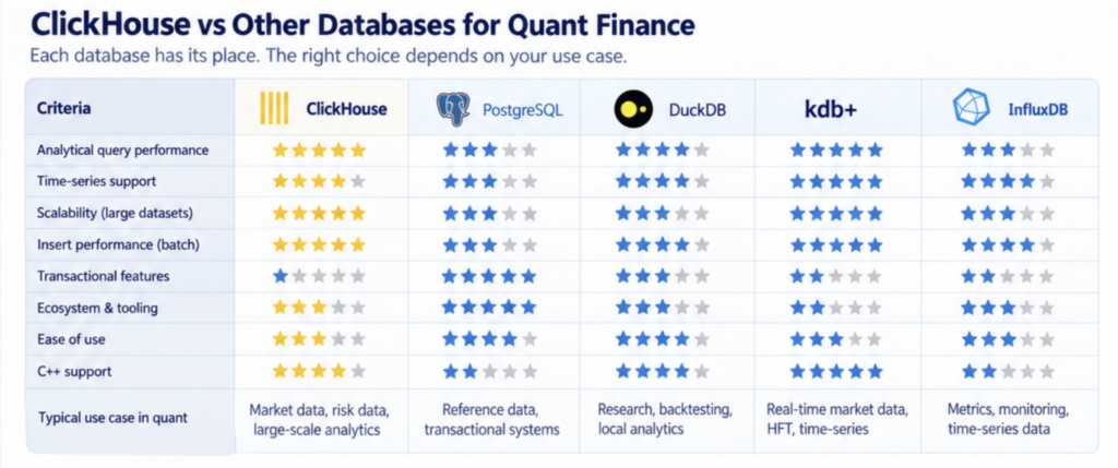
So, how to conclude? Maybe with a comparison with other databases and a list of strengths/weaknesses.

Different systems are optimized for different workloads. PostgreSQL is a strong general-purpose relational database, DuckDB is excellent for local analytical work, kdb+ has a long history in high-performance market data, and InfluxDB is designed around time-series workloads.

ClickHouse sits in a different part of the spectrum. Its main strength is large-scale analytical processing: scanning, filtering and aggregating very large datasets quickly.

The comparison below is therefore not about choosing a universal winner, but about understanding where ClickHouse fits relative to other common database choices in quantitative systems.

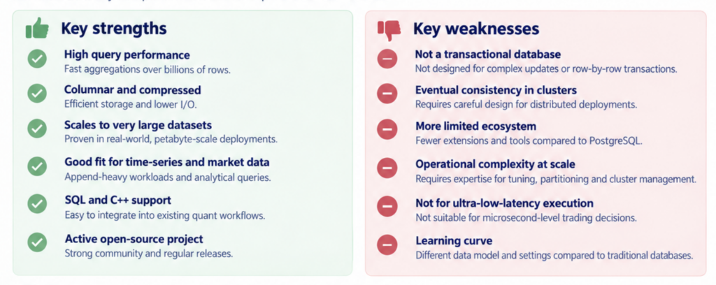
The summary below highlights the main strengths and weaknesses of ClickHouse and helps place it in the broader context of quantitative finance infrastructure:

September 6, 2026 0 comments
Order Book C++
Data StructuresInterviewPerformance

Data Structures for Order Book: std::map, std::unordered_map, or std::vector?

by cppforquants July 12, 2026

Ask a C++ developer to design a limit order book, and you will almost always get the same answer: std::map<Price, Level>. It is the answer every tutorial gives, the answer that passes the coding screen, and the answer that feels obviously right: an order book is a collection of price levels that must stay sorted, and std::map is the sorted container. Case closed.

Except that if you look at how production trading systems are actually built, you will struggle to find a red-black tree anywhere near the hot path. The container that “obviously” fits the problem is quietly absent from the systems where the problem matters most.

This article explains why, by putting three candidates through the same test: std::unordered_map, std::map, and — the one nobody suggests in interviews — std::vector.


1.Refresher on std::map, std::unordered_map and std::vectors

What are maps?

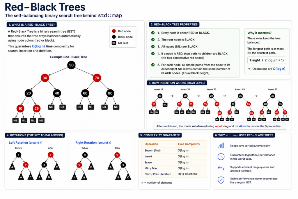
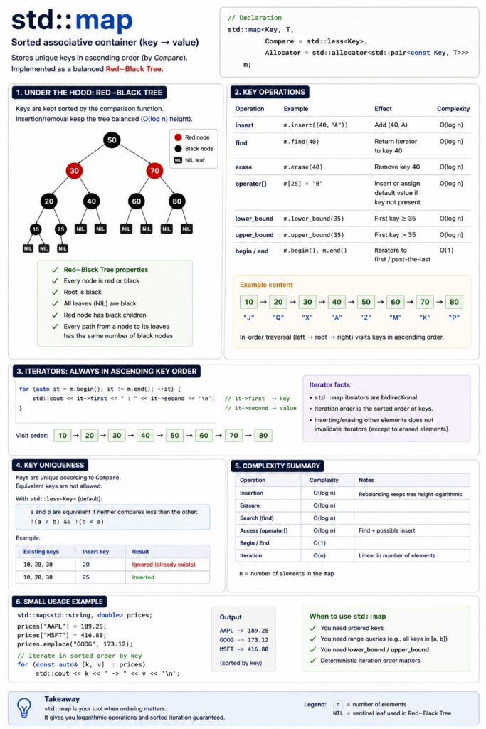
A std::map is a sorted associative container storing key-value pairs with unique keys, typically implemented as a red-black tree.

Lookups, insertions, and deletions are all O(log n), and iterating gives you elements in key order.

A good summary video:

What are unordered maps?

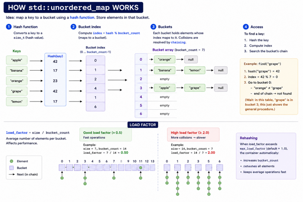
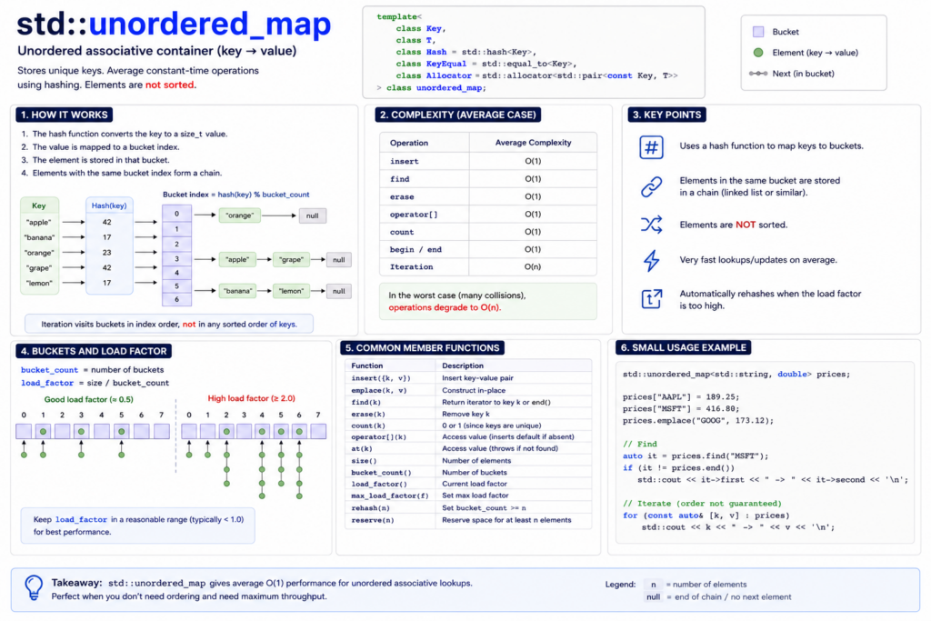
A std::unordered_map is a hash table storing key-value pairs with unique keys but no ordering guarantee.

Average O(1) lookup, insert, and erase, degrading to O(n) in the worst case (hash collisions).

The trade-offs: it needs a hash function for the key type, iteration order is unspecified, and the node-based bucket implementation means pointer chasing that can hurt cache performance — which is why HFT code often reaches for open-addressing alternatives like absl::flat_hash_map.

What are vectors?


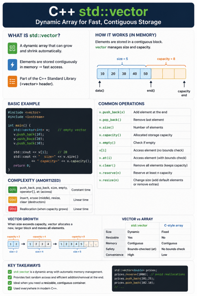
std::vector is C++’s dynamic array: it stores elements in contiguous memory, gives fast indexed access, and automatically grows when you add more elements.

How to use them to create an order book? But, by the way, what’s an order book?


2. Refresher on order books

An order book is the mechanism that allows a market to match buyers and sellers.

A trader can send:

Buy 100 shares at 99.98
Sell 200 shares at 100.02
Buy 50 shares at market
Cancel order #123
Modify order #456

The exchange maintains the book and decides what happens next.

An order book is the live list of buyers and sellers for a financial instrument.

At first, it is often shown as a table:

Bid SizeBid PriceAsk PriceAsk Size
500 99.98 100.02 300
1,200 99.97 100.03 700
800 99.96 100.04 1,500

The bid side represents buyers.
The ask side represents sellers.

Here, “size” means quantity.

So:

500 at 99.98 means buyers want to buy 500 shares at 99.98.
300 at 100.02 means sellers want to sell 300 shares at 100.02.

Each row is also called a price level.

Level 1 is the best available price on each side:

Level 1 bid = 99.98 x 500
Level 1 ask = 100.02 x 300

Level 2 is the next best price:

Level 2 bid = 99.97 x 1,200
Level 2 ask = 100.03 x 700

Level 3 is the next one after that:

Level 3 bid = 99.96 x 800
Level 3 ask = 100.04 x 1,500

A more natural way to visualize the book is vertically:

            ASK SIDE

Level 3     100.04 x 1,500
Level 2     100.03 x 700
Level 1     100.02 x 300     <- best ask

            spread = 0.04

Level 1      99.98 x 500     <- best bid
Level 2      99.97 x 1,200
Level 3      99.96 x 800

            BID SIDE

The best bid is the highest price someone is willing to buy at.
The best ask is the lowest price someone is willing to sell at.

3. Model an Order Book in C++: Various Attempts

Attempt 1: hash the price levels with std::unordered_map

The message flow suggests an obvious first design. Cancels dominate, and cancels are lookups — so we optimize for lookup. A hash map from price to level gives us O(1) access to any level, and std::unordered_map is sitting right there in the standard library:

cpp

std::unordered_map<Price, Level> bids_;
std::unordered_map<Price, Level> asks_;

Adds are O(1). Cancels are O(1). Modifies are O(1). On paper we’ve made the dominant operations constant-time, and for a few minutes this feels like a solved problem.

Then we implement best_bid().

There is no “first element” in a hash map. Hashing deliberately destroys ordering — that’s what makes it fast — so the only way to find the highest bid is to scan every populated level. The book’s single most frequent query, the one strategy code calls on effectively every tick, has become O(n) over the entire side. Depth walks are worse: there’s no notion of “the next level down” at all; we’d re-scan or sort on demand.

We didn’t build a slow order book. We built something that structurally isn’t an order book. An order book’s defining property is that its levels are ordered — it’s in the name — and we chose the one container whose entire design premise is discarding order. The lookup speed was real, but we optimized the operation that was never going to be the bottleneck and broke the one that defines the product.

Attempt 2: the tree with std::map

So ordering is non-negotiable. The standard library’s ordered associative container is std::map, a red-black tree, and it fixes everything the hash map broke:

std::map<Price, Level, std::greater<Price>> bids_;  // begin() is best bid
std::map<Price, Level> asks_;                        // begin() is best ask

Best bid is bids_.begin() — O(1). Depth walks are in-order traversal. Adds, cancels, and modifies are O(log n), and with a few hundred populated levels, log n is under ten comparisons. This is the textbook answer, it’s correct, and it’s what most order book implementations you’ll find online actually use.

Now replay a day of market data through it and watch what the hardware does.

A full implementation of that version that would make you pass the quant interview in C++ has been proposed in our first article on order books:

using OrderId   = uint64_t;
using Qty       = int64_t;        // signed for partial fills math
using Px       = int64_t;         // price in ticks
enum Side { Buy, Sell };

struct Order {
  OrderId id;
  Side side;
  Px price;
  Qty qty;            // remaining
  uint64_t ts;        // exchange/seq time for tie-breaks
  // intrusive list pointers for O(1) erase
  Order* prev = nullptr;
  Order* next = nullptr;
};

struct Level {
  Px price;
  Order* head = nullptr;
  Order* tail = nullptr;
  inline void push_back(Order* o);
  inline void erase(Order* o);
  bool empty() const { return head == nullptr; }
};

// price → level; bids need descending, asks ascending
using BookSide = std::map<Px, Level, std::greater<Px>>;     // bids
using BookSideAsk = std::map<Px, Level, std::less<Px>>;     // asks

struct OrderBook {
  BookSide bids;
  BookSideAsk asks;
  std::unordered_map<OrderId, Order*> by_id;  // direct handle for cancel/replace

  // API
  void add_limit(OrderId id, Side side, Px px, Qty qty, uint64_t ts);
  void cancel(OrderId id);
  void replace(OrderId id, Px new_px, Qty new_qty, uint64_t ts); // cancel+add semantics
  void match_market(Side side, Qty qty);
  // helpers
  Level& level(BookSide& s, Px px);
  Level& level(BookSideAsk& s, Px px);
};

Attempt 3: keep it sorted, make it contiguous

If pointer chasing is the disease, contiguity is the cure. A sorted std::vector<Level> with binary search keeps the ordering guarantee but lays every level out in a single flat allocation:

cpp

std::vector<Level> bids_;  // sorted; back() is best bid

Lookup is std::lower_bound — still O(log n) comparisons, but now the search touches a handful of cache lines in one array instead of five scattered heap nodes, and the hardware prefetcher can see where we’re going. Best bid is back(). Insertion of a new level requires shifting elements — O(n) in theory — but here the workload rescues us: adds cluster near the touch, so if the vector is sorted with the best price at the back, the memmove is almost always a few elements. In practice this structure embarrasses the tree on a realistic feed.

And yet, benchmark it honestly and there’s a residue we can’t scrub out. Every operation still begins with a search — a binary search is a series of dependent loads, each one’s address unknown until the previous compare resolves, so the pipeline stalls on each step. We’ve made searching cheap. We haven’t asked whether we need to search at all.

Attempt 4: stop searching

Every structure so far has treated the price as an opaque key — something to hash, compare, or binary-search for. But a price in a limit order book is none of those things. Exchanges don’t accept arbitrary prices: every instrument trades on a fixed grid, an integer number of ticks. Two consecutive price levels don’t just happen to be close — they differ by exactly one tick, always. That’s not a statistical tendency we can exploit; it’s a hard constraint the venue enforces on every order.

Once you see prices as grid positions rather than keys, the search problem dissolves. If we know the tick size and pick an anchor price for index zero, then the level for any price isn’t something we find — it’s something we compute.

index = (price − anchor) / tick

One subtraction, one division by a constant, one indexed load into a flat array. No hash function, no comparisons, no dependent loads waiting on the previous step to resolve. The lookup that cost the tree five scattered pointer dereferences and cost the sorted vector a pipeline-stalling binary search is now cheaper than either structure’s first step.

4. A Proposition of Implementation for Attempt 4

In the approach we’re presenting, prices are ticks on a fixed grid, so the book is a flat array of price levels where a price is converted to an index by one subtraction — no hashing, no tree, no search — with a cached best index and each level holding a FIFO of pool-allocated orders linked intrusively.

Adds, cancels, and executions each cost an arithmetic index or an O(1) ID lookup plus an O(1) unlink, touching two or three cache lines and zero heap allocations on the hot path.

Let’s start with an order_book.hpp:

// order_book.hpp — tick-indexed limit order book
//
// Design (see article): contiguous array of price levels indexed by tick
// offset, intrusive doubly-linked FIFO per level, pre-allocated order pool,
// open-addressing map for OrderId -> Order*. Zero heap allocation on the
// hot path after construction.
//
// Conventions:
//   - Price is an integer number of ticks (scale at the feed decoder).
//   - OrderId 0 and ~0 are reserved (empty / tombstone sentinels in IdMap).

#pragma once

#include <cassert>
#include <cstddef>
#include <cstdint>
#include <vector>

using Price   = std::int64_t;
using Qty     = std::int64_t;
using OrderId = std::uint64_t;

enum class Side : std::uint8_t { Bid, Ask };

// ---------------------------------------------------------------------------
// Order: 64 bytes, cache-line aligned. prev/next are intrusive — the order
// *is* its own list node, so joining/leaving a level allocates nothing.
// ---------------------------------------------------------------------------
struct alignas(64) Order {
    OrderId id;
    Qty     qty;
    Price   price;
    Side    side;
    Order*  prev;
    Order*  next;
};
static_assert(sizeof(Order) == 64, "one order per cache line");

// ---------------------------------------------------------------------------
// OrderPool: all orders live in one contiguous slab allocated at startup.
// alloc/release are a free-list push/pop — no new/delete on the hot path.
// ---------------------------------------------------------------------------
class OrderPool {
public:
    explicit OrderPool(std::size_t capacity) : slots_(capacity) {
        free_.reserve(capacity);
        for (std::size_t i = capacity; i-- > 0;)
            free_.push_back(&slots_[i]);
    }

    Order* alloc() {
        assert(!free_.empty() && "pool exhausted — size it to the session");
        Order* o = free_.back();
        free_.pop_back();
        return o;
    }

    void release(Order* o) { free_.push_back(o); }

private:
    std::vector<Order>  slots_;
    std::vector<Order*> free_;
};

// ---------------------------------------------------------------------------
// Level: FIFO queue of resting orders at one price. head is oldest (first to
// fill), tail is where adds append — price-time priority falls out of the
// list order. total_qty is maintained incrementally so top-of-book snapshots
// never walk the list.
// ---------------------------------------------------------------------------
struct Level {
    Order* head      = nullptr;
    Order* tail      = nullptr;
    Qty    total_qty = 0;

    bool empty() const { return head == nullptr; }

    void push_back(Order* o) {
        o->prev = tail;
        o->next = nullptr;
        if (tail) tail->next = o; else head = o;
        tail = o;
        total_qty += o->qty;
    }

    // O(1) given the order pointer — no search. This is why cancels, the
    // dominant message type, stay cheap.
    void unlink(Order* o) {
        if (o->prev) o->prev->next = o->next; else head = o->next;
        if (o->next) o->next->prev = o->prev; else tail = o->prev;
        total_qty -= o->qty;
    }
};

// ---------------------------------------------------------------------------
// BookSide: the tick-indexed array. Price -> level is one subtraction and
// one indexed load; no hashing, no comparisons, no pointer chasing.
// best_ caches the top of book; when the top level empties we scan linearly
// toward the interior — adjacent prices are adjacent cache lines, and the
// next populated level is almost always within a few ticks.
// ---------------------------------------------------------------------------
template <bool IsBid>
class BookSide {
public:
    static constexpr std::size_t kLevels = std::size_t{1} << 16;
    static constexpr std::size_t kNone   = ~std::size_t{0};

    explicit BookSide(Price anchor)
        : levels_(kLevels), anchor_(anchor) {}

    void add(Order* o) {
        const std::size_t idx = index(o->price);
        levels_[idx].push_back(o);
        if (best_ == kNone || better(idx, best_)) best_ = idx;
    }

    void remove(Order* o) {
        const std::size_t idx = index(o->price);
        levels_[idx].unlink(o);
        if (idx == best_ && levels_[idx].empty()) advance_best();
    }

    void reduce(Order* o, Qty by) {
        o->qty -= by;
        levels_[index(o->price)].total_qty -= by;
    }

    bool  empty()      const { return best_ == kNone; }
    Price best_price() const { return anchor_ + static_cast<Price>(best_); }
    Qty   best_qty()   const { return levels_[best_].total_qty; }
    const Order* best_order() const { return levels_[best_].head; }

private:
    std::size_t index(Price p) const {
        assert(p >= anchor_ &&
               static_cast<std::size_t>(p - anchor_) < kLevels &&
               "price outside book range — re-anchor on the slow path");
        return static_cast<std::size_t>(p - anchor_);
    }

    static bool better(std::size_t a, std::size_t b) {
        if constexpr (IsBid) return a > b;   // best bid = highest price
        else                 return a < b;   // best ask = lowest price
    }

    void advance_best() {
        if constexpr (IsBid) {
            while (best_ != 0) {
                --best_;
                if (!levels_[best_].empty()) return;
            }
        } else {
            while (best_ + 1 < kLevels) {
                ++best_;
                if (!levels_[best_].empty()) return;
            }
        }
        best_ = kNone;   // side is empty
    }

    std::vector<Level> levels_;   // one flat allocation, made once
    Price              anchor_;   // price at index 0
    std::size_t        best_ = kNone;
};

// ---------------------------------------------------------------------------
// IdMap: OrderId -> Order*, open addressing with linear probing. Flat slot
// array — one hash, then a short contiguous probe. Sized 2x expected load
// at construction; erases leave tombstones (fine for a trading session,
// rebuild between sessions if reusing).
// ---------------------------------------------------------------------------
// ---------------------------------------------------------------------------
// IdMap: OrderId -> Order*, open addressing with linear probing. Flat slot
// array — one hash, then a short contiguous probe. Sized 2x expected load
// at construction; erases leave tombstones (fine for a trading session,
// rebuild between sessions if reusing).
// ---------------------------------------------------------------------------
class IdMap {
public:
    explicit IdMap(std::size_t expected) {
        std::size_t cap = 1;
        while (cap < expected * 2) cap <<= 1;
        slots_.assign(cap, Slot{kEmpty, nullptr});
        mask_ = cap - 1;
    }

    void insert(OrderId id, Order* o) {
        std::size_t i = hash(id) & mask_;
        while (slots_[i].key != kEmpty && slots_[i].key != kTomb)
            i = (i + 1) & mask_;
        slots_[i] = Slot{id, o};
    }

    Order* find(OrderId id) const {
        std::size_t i = hash(id) & mask_;
        while (slots_[i].key != kEmpty) {
            if (slots_[i].key == id) return slots_[i].val;
            i = (i + 1) & mask_;
        }
        return nullptr;
    }

    void erase(OrderId id) {
        std::size_t i = hash(id) & mask_;
        while (slots_[i].key != kEmpty) {
            if (slots_[i].key == id) {
                slots_[i].key = kTomb;
                slots_[i].val = nullptr;
                return;
            }
            i = (i + 1) & mask_;
        }
    }

private:
    static constexpr OrderId kEmpty = 0;
    static constexpr OrderId kTomb  = ~OrderId{0};

    struct Slot { OrderId key; Order* val; };

    static std::size_t hash(OrderId id) {   // splitmix64 finalizer
        std::uint64_t x = id;
        x ^= x >> 33; x *= 0xff51afd7ed558ccdULL;
        x ^= x >> 33; x *= 0xc4ceb9fe1a85ec53ULL;
        x ^= x >> 33;
        return static_cast<std::size_t>(x);
    }

    std::vector<Slot> slots_;
    std::size_t       mask_;
};

// ---------------------------------------------------------------------------
// OrderBook: ties the pieces together. The three feed-driven mutations map
// onto it directly:
//   Add     -> pool alloc, arithmetic index, list append   (0 allocations)
//   Cancel  -> id lookup, O(1) unlink, pool release        (0 allocations)
//   Execute -> id lookup, reduce or remove                 (0 allocations)
// ---------------------------------------------------------------------------
class OrderBook {
public:
    struct Quote { Price price; Qty qty; bool valid; };

    OrderBook(Price anchor, std::size_t max_live_orders)
        : bids_(anchor), asks_(anchor),
          pool_(max_live_orders), ids_(max_live_orders) {}

    void add(OrderId id, Side side, Price price, Qty qty) {
        Order* o = pool_.alloc();
        *o = Order{id, qty, price, side, nullptr, nullptr};
        if (side == Side::Bid) bids_.add(o); else asks_.add(o);
        ids_.insert(id, o);
    }

    void cancel(OrderId id) {
        if (Order* o = ids_.find(id)) remove(o);
    }

    // Execution reported by the feed against a resting order.
    void execute(OrderId id, Qty exec_qty) {
        Order* o = ids_.find(id);
        if (!o) return;
        if (exec_qty >= o->qty) {
            remove(o);
        } else if (o->side == Side::Bid) {
            bids_.reduce(o, exec_qty);
        } else {
            asks_.reduce(o, exec_qty);
        }
    }

    Quote best_bid() const {
        return bids_.empty() ? Quote{0, 0, false}
                             : Quote{bids_.best_price(), bids_.best_qty(), true};
    }

    Quote best_ask() const {
        return asks_.empty() ? Quote{0, 0, false}
                             : Quote{asks_.best_price(), asks_.best_qty(), true};
    }

private:
    void remove(Order* o) {
        if (o->side == Side::Bid) bids_.remove(o); else asks_.remove(o);
        ids_.erase(o->id);
        pool_.release(o);
    }

    BookSide<true>  bids_;
    BookSide<false> asks_;
    OrderPool       pool_;
    IdMap           ids_;
};

How to test this approach?

Create a demo.cpp:

#include "order_book.hpp"
#include <cstdio>

static void print_top(const OrderBook& book, const char* tag) {
    auto b = book.best_bid();
    auto a = book.best_ask();
    std::printf("%-28s  bid: ", tag);
    if (b.valid) std::printf("%lld x %lld", (long long)b.qty, (long long)b.price);
    else         std::printf("--");
    std::printf("   ask: ");
    if (a.valid) std::printf("%lld x %lld", (long long)a.qty, (long long)a.price);
    else         std::printf("--");
    std::printf("\n");
}

int main() {
    // Anchor at tick 10'000, capacity for 1M live orders.
    OrderBook book(/*anchor=*/10'000, /*max_live_orders=*/1'000'000);

    book.add(1, Side::Bid, 10'100, 500);
    book.add(2, Side::Bid, 10'101, 300);   // better bid
    book.add(3, Side::Bid, 10'101, 200);   // joins queue behind id 2
    book.add(4, Side::Ask, 10'103, 400);
    book.add(5, Side::Ask, 10'102, 250);   // better ask
    print_top(book, "after adds");

    book.cancel(2);                        // partial drain of best bid level
    print_top(book, "cancel id 2");

    book.cancel(3);                        // best bid level empties -> scan inward
    print_top(book, "cancel id 3");

    book.execute(5, 100);                  // partial execution at best ask
    print_top(book, "execute 100 vs id 5");

    book.execute(5, 150);                  // fills remainder -> level empties
    print_top(book, "execute 150 vs id 5");

    book.cancel(1);
    book.cancel(4);
    print_top(book, "book emptied");

    return 0;
}

Let’s compile and run:

g++ -std=c++20 -O2 -Wall -Wextra -o demo demo.cpp && ./demo

Which gives:

after adds                    bid: 500 x 10101   ask: 250 x 10102
cancel id 2                   bid: 200 x 10101   ask: 250 x 10102
cancel id 3                   bid: 500 x 10100   ask: 250 x 10102
execute 100 vs id 5           bid: 500 x 10100   ask: 150 x 10102
execute 150 vs id 5           bid: 500 x 10100   ask: 400 x 10103
book emptied                  bid: --   ask: --
July 12, 2026 0 comments
Best C++ libraries for parallel processing
LibrariesPerformance

Best C++ Libraries for Parallel Programming

by cppforquants June 11, 2026

One of the most important topics in C++ is parallel programming. While the C++ Standard Library provides foundational concurrency primitives such as std::thread, std::mutex, and std::async, or more recent SIMD additions, many real-world applications benefit from higher-level abstractions. Modern parallel programming libraries offer task schedulers, work-stealing runtimes, dependency graphs, distributed execution models, and performance-portable frameworks that dramatically simplify the development of scalable systems. What are the best C++ libraries for parallel programming?

1. OpenMP

OpenMP (Open Multi-Processing) is an open standard for shared-memory parallel programming that allows developers to parallelize code using compiler directives, library routines, and environment variables. It’s one of the best C++ libraries for parallel programming.

It was first introduced in 1997 by the OpenMP Architecture Review Board (ARB), a consortium of hardware and software companies that included organizations such as Intel, IBM, Hewlett-Packard, and others. The goal was to create a portable and vendor-neutral standard for exploiting multiple CPU cores on shared-memory systems.

Monte Carlo pricing is a classic example of an embarrassingly parallel workload. By distributing simulation paths across multiple CPU cores, OpenMP can significantly reduce execution times with only a few additional lines of code.

Let’s create a “monte_carlo.cpp” file:

#include <omp.h>
#include <cmath>
#include <random>
#include <vector>
#include <iostream>

double simulate_option_price(
    double spot,
    double strike,
    double rate,
    double vol,
    double maturity,
    int num_paths)
{
    double payoff_sum = 0.0;

    #pragma omp parallel
    {
        std::mt19937 rng(42 + omp_get_thread_num());
        std::normal_distribution<> normal(0.0, 1.0);

        double local_sum = 0.0;

        #pragma omp for
        for (int i = 0; i < num_paths; ++i)
        {
            double z = normal(rng);

            double st =
                spot * std::exp(
                    (rate - 0.5 * vol * vol) * maturity +
                    vol * std::sqrt(maturity) * z);

            local_sum += std::max(st - strike, 0.0);
        }

        #pragma omp atomic
        payoff_sum += local_sum;
    }

    return std::exp(-rate * maturity) * payoff_sum / num_paths;
}

int main()
{
    double price = simulate_option_price(
        100.0,
        100.0,
        0.05,
        0.20,
        1.0,
        10'000'000);

    std::cout << "Option Price: " << price << '\n';
}

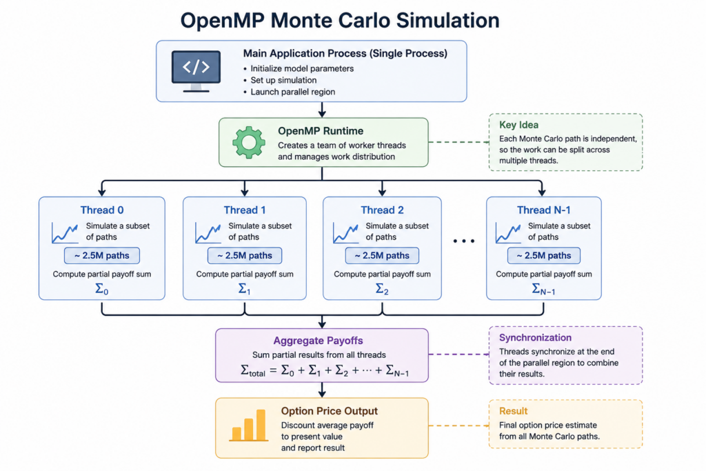
In the code above, each thread is responsible for a portion of the Monte Carlo simulations. Because individual simulation paths are completely independent, they can be executed concurrently on multiple CPU cores before their results are aggregated into a final option price estimate.
Compiling the Example

OpenMP is implemented through compiler support rather than as a standalone library. When the compiler encounters OpenMP directives such as #pragma omp parallel or #pragma omp for, it generates the necessary multithreaded code and links against the OpenMP runtime.

To compile the example using GCC:

g++ -O3 -fopenmp monte_carlo.cpp -o monte_carlo

The -fopenmp flag enables OpenMP support and links the OpenMP runtime library. Without this flag, the compiler will ignore the OpenMP directives and execute the code sequentially.

On macOS, the default Apple Clang compiler does not always include OpenMP support. In this case, developers typically install LLVM or GCC through Homebrew and compile the program using an OpenMP-enabled compiler.

Then execute the code:

./monte_carlo

The simulation above will be split on different threads before an aggregation step:

2.oneTBB

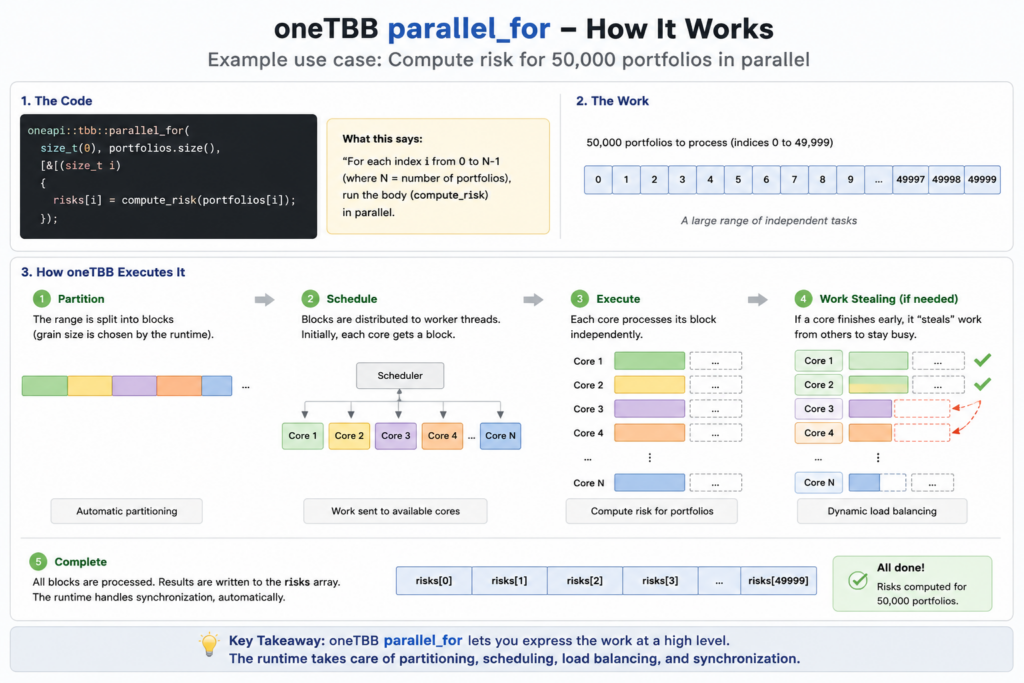
oneTBB (formerly Intel Threading Building Blocks) is a task-based parallel programming library created by Intel and first released in 2006. Rather than managing threads directly, developers express work as tasks, allowing oneTBB’s scheduler to efficiently distribute computation across multiple CPU cores.

Widely used in high-performance computing, quantitative finance, and scientific applications, oneTBB provides parallel algorithms, concurrent containers, and a work-stealing scheduler designed to simplify scalable multicore development.

A bank needs to recompute a risk metric for 50,000 portfolios after a market move. Since each portfolio can be processed independently, the workload is naturally parallel. Instead of manually creating and managing threads, oneTBB distributes the portfolios across available CPU cores and balances the work automatically.

#include <oneapi/tbb/parallel_for.h>
#include <vector>

struct Portfolio
{
    std::string portfolio_id;
    std::vector<double> trade_dv01s;
};

double compute_risk(const Portfolio& portfolio)
{
    double dv01 = 0.0;

    for(double trade_dv01 : portfolio.trade_dv01s)
    {
        dv01 += trade_dv01;
    }

    return dv01;
}

int main()
{
    std::vector<Portfolio> portfolios(50000);
    std::vector<double> risks(portfolios.size());

    oneapi::tbb::parallel_for(
        size_t(0),
        portfolios.size(),
        [&](size_t i)
        {
            risks[i] = compute_risk(portfolios[i]);
        });

    return 0;
}

In this example, each portfolio can be evaluated independently, making the workload embarrassingly parallel. The parallel_for algorithm automatically divides the portfolio universe into smaller chunks and schedules them across available CPU cores. Unlike traditional thread-based approaches, developers do not need to manage thread creation, synchronization, or load balancing manually. This allows applications to scale efficiently on multicore systems while keeping the code concise and maintainable.

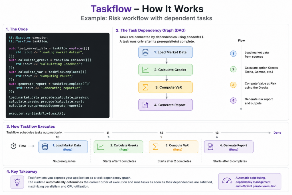
3.TaskFlow

Taskflow is a modern C++ parallel programming library that allows developers to express applications as task dependency graphs (DAGs) rather than individual threads or loops. It automatically schedules tasks, manages dependencies, and executes workflows efficiently across available CPU cores, making it particularly well-suited for data pipelines, simulations, and complex computational workflows. Taskflow is one the best C++ libraries for parallel programming.

The project was first presented publicly in 2019 as “Cpp-Taskflow: Fast Task-Based Parallel Programming Using Modern C++”.


The following example models a simple risk analytics pipeline. Market data must be loaded before risk calculations can begin, while independent calculations can run in parallel. Once all computations are complete, a report is generated

#include <taskflow/taskflow.hpp>

int main() {

    tf::Executor executor;
    tf::Taskflow taskflow;

    auto load_market_data = taskflow.emplace([]{
        std::cout << "Loading market data\n";
    });

    auto calculate_greeks = taskflow.emplace([]{
        std::cout << "Calculating Greeks\n";
    });

    auto calculate_var = taskflow.emplace([]{
        std::cout << "Computing VaR\n";
    });

    auto generate_report = taskflow.emplace([]{
        std::cout << "Generating report\n";
    });

    load_market_data.precede(calculate_greeks);
    calculate_greeks.precede(calculate_var);
    calculate_var.precede(generate_report);

    executor.run(taskflow).wait();
}

Unlike OpenMP and oneTBB, which primarily focus on parallel loops and tasks, Taskflow allows developers to express entire applications as dependency graphs. Independent tasks can execute concurrently, while dependent tasks automatically wait for their prerequisites to complete. This approach is particularly useful for data pipelines, machine learning workflows, risk calculations, and other complex computational processes.

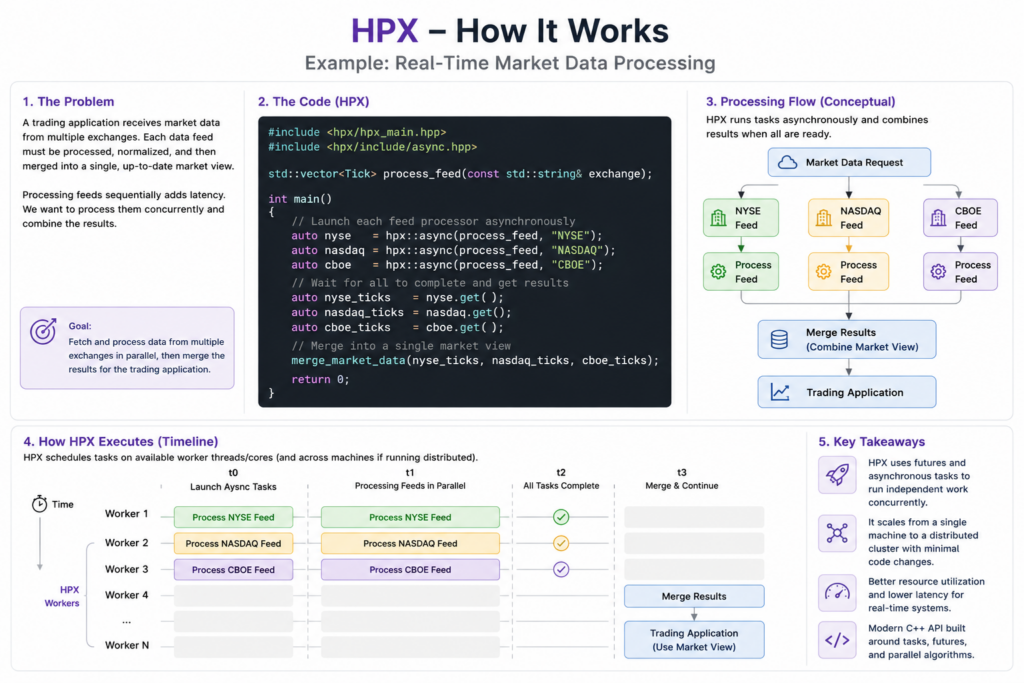
4.HPX

HPX is a modern C++ runtime system designed for scalable parallel and distributed applications. It extends the C++ standard library with asynchronous programming primitives such as futures, parallel algorithms, and task scheduling, allowing developers to write code that can scale from a laptop to a large computing cluster with minimal changes.

Typical Use Cases

  • Scientific computing
  • Distributed simulations
  • Numerical methods
  • Large-scale graph processing
  • HPC applications
  • Quantitative finance workloads requiring cluster-scale execution

Imagine a trading platform receives market data from multiple exchanges. Instead of processing each feed sequentially, HPX can launch asynchronous tasks and combine the results once all feeds have been processed.

#include <hpx/hpx_main.hpp>
#include <hpx/include/async.hpp>

std::vector<Tick> process_feed(const std::string& exchange);

int main()
{
    auto nyse = hpx::async(process_feed, "NYSE");
    auto nasdaq = hpx::async(process_feed, "NASDAQ");
    auto cboe = hpx::async(process_feed, "CBOE");

    auto nyse_ticks = nyse.get();
    auto nasdaq_ticks = nasdaq.get();
    auto cboe_ticks = cboe.get();

    merge_market_data(
        nyse_ticks,
        nasdaq_ticks,
        cboe_ticks
    );
}

In this example, market data from multiple exchanges is processed concurrently using HPX futures. Each feed is handled asynchronously, allowing the application to utilize available computing resources efficiently while avoiding unnecessary blocking. Once all tasks complete, the results are merged into a unified market view.

In summary, HPX is one of the best C++ libraries for parallel programming!

5. A Summary of Pros and Cons

The libraries covered in this article address different parallel programming challenges, from simple loop parallelism to task scheduling, workflow orchestration, and distributed execution. The best choice depends on the complexity of your workload and how much control you need over execution.

LibraryStrengthsWeaknesses
OpenMPEasy to learn, simple loop parallelism, broad compiler supportLimited flexibility for complex task dependencies
oneTBBTask-based programming, automatic load balancing, scalable runtimeMore concepts to learn than OpenMP
TaskflowElegant workflow graphs (DAGs), intuitive dependency managementSmaller ecosystem and fewer learning resources
HPXFutures, asynchronous execution, distributed computing supportSteeper learning curve and more advanced programming model

Choosing the Right Library

  • OpenMP is ideal when you need to parallelize loops with minimal code changes.
  • oneTBB is a strong choice for applications composed of many independent tasks.
  • Taskflow excels at modelling complex workflows with explicit dependencies.
  • HPX is designed for highly scalable asynchronous applications that may span multiple machines.

In short: OpenMP focuses on loops, oneTBB on tasks, Taskflow on workflows, and HPX on asynchronous and distributed execution. Together, they represent a progression from straightforward multicore programming to advanced parallel and distributed systems.

June 11, 2026 0 comments
LibrariesPerformance

Detecting Arithmetic Overflow in C++: Finance-Safe Arithmetic

by cppforquants April 2, 2026

Somewhere in a production pricing engine, a 32-bit integer silently wraps around during a notional accumulation, a Greeks ladder miscounts its buckets, or a risk aggregation quietly produces a number that is just slightly wrong — and nobody notices until the end-of-day reconciliation, or worse, until a trader calls. Arithmetic overflow is one of the oldest bugs in systems programming, yet in C++ it carries a particularly sharp edge: signed overflow is undefined behaviour, meaning the compiler is not only permitted to produce a wrong answer, it is permitted to optimise away the very branch you wrote to catch it. In latency-sensitive financial code, where you’re burning through millions of option valuations or margin calculations per second, this is not a theoretical concern.


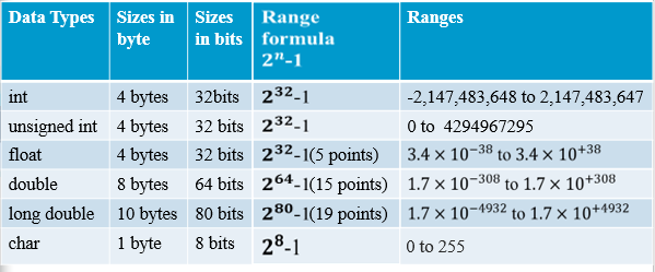
Ranges for data types in C++

The good news is that modern C++ — and GCC/Clang long before the standard caught up — gives you a near-zero-cost escape hatch: __builtin_add_overflow, __builtin_mul_overflow, and their family members. These compiler intrinsics lower directly to native overflow-checking instructions (think jo on x86 or the carry-flag variants), producing branch-predictable, exception-free code that slots cleanly into hot loops without touching the exception machinery or sacrificing throughput.

What Is Arithmetic overflow detection with __builtin_add_overflow / std::add_overflow (and the upcoming contracts alternative)?

Signed integer overflow in C++ is undefined behavior — the compiler is legally allowed to assume it never happens, which means optimizers can and do eliminate overflow checks written naively with if (a + b < a). This isn’t a theoretical concern; GCC and Clang routinely delete such guards under -O2. The problem demands a solution that is both correct and efficient.

GCC and Clang expose __builtin_add_overflow(a, b, &result), along with __builtin_sub_overflow and __builtin_mul_overflow. These builtins perform the arithmetic in the mathematical integers, store the wrapped result in *result, and return true if the true value doesn’t fit in the result type. Crucially, the type of result drives the overflow semantics — mixing signed and unsigned types works predictably because the check is against the destination type, not the operands. MSVC offers UIntAdd, IntAdd, etc. from <intsafe.h> for similar unsigned coverage, though without the same generality.

int a = INT_MAX, b = 1, result;
if (__builtin_add_overflow(a, b, &result)) {
    // overflow detected; result holds the wrapped value
}

Under the hood, modern compilers lower these to a single add + jo/jno (overflow flag check) on x86, or adds + branch on ARM — one instruction overhead, no undefined behavior.

C++26 is expected to introduce std::add_overflow and friends in <numeric>, standardizing the API surface across implementations. Separately, the Contracts proposal ([[pre]], [[post]]) enables expressing overflow preconditions declaratively, though contracts terminate rather than branch, making them unsuitable for recoverable overflow handling.

Common pitfalls: assuming the builtin is only for int — it works on any integral type including size_t. Forgetting that the result pointer type governs overflow semantics leads to subtle bugs when mixing widths. Finally, don’t use these builtins on floating-point; they’re strictly integral.

Practical Use Case in Finance

A high-frequency trading order aggregation engine must sum large 64-bit notional values across thousands of fills per second. Silent integer overflow here means a corrupted position — a catastrophic risk event.

Setup: Each fill carries a notional (quantity × price in cents). We accumulate these into a running total_notional. With values potentially in the billions, overflow is a real threat that must be caught immediately, not discovered during end-of-day reconciliation.

#include <cstdint>
#include <stdexcept>
#include <iostream>
#include <vector>

// Represents a single trade fill
struct Fill {
    int64_t notional_cents; // qty * price in cents (can be large)
};

// Accumulates notional with overflow protection.
// Uses GCC/Clang __builtin_add_overflow; on MSVC use safeint or manual check.
int64_t aggregate_notional(const std::vector<Fill>& fills) {
    int64_t total = 0;

    for (const auto& fill : fills) {
        int64_t next = 0;

        // __builtin_add_overflow returns true if overflow would occur,
        // storing the wrapped result in `next` (which we discard on error).
        if (__builtin_add_overflow(total, fill.notional_cents, &next)) {
            throw std::overflow_error(
                "Notional accumulation overflowed int64 — "
                "halt aggregation, alert risk desk immediately."
            );
        }

        total = next;
    }
    return total;
}

int main() {
    // Simulate fills approaching int64 limits
    int64_t near_max = INT64_MAX - 1000;
    std::vector<Fill> fills = {
        {near_max},
        {500},   // fine
        {600},   // this tips over the edge
    };

    try {
        int64_t result = aggregate_notional(fills);
        std::cout << "Total notional: " << result << " cents\n";
    } catch (const std::overflow_error& e) {
        std::cerr << "[RISK ALERT] " << e.what() << '\n';
        // In production: publish alert, reject batch, trigger circuit breaker
    }
}

What this demonstrates: __builtin_add_overflow performs the addition and overflow detection in a single CPU instruction (ADD + JO on x86), with zero overhead on the happy path — critical for a hot loop. Compared to pre-checking with INT64_MAX - a < b, it is both safer and faster. The upcoming C++26 Contracts feature ([[pre: ...]]) will allow expressing these invariants declaratively at function boundaries, but __builtin_add_overflow remains the practical tool today for inline arithmetic guards in latency-sensitive paths.

Learn More: A Video Worth Watching

Understanding integer overflow vulnerabilities is crucial for developers working in quantitative finance, where precision and correctness directly impact trading systems and risk calculations. This video from Marcus Hutchins provides an accessible introduction to how binary integers work and the mechanics behind overflow conditions—foundational knowledge that contextualizes why C++ provides built-in overflow detection tools like __builtin_add_overflow and the standardized std::add_overflow (coming in C++26).
For quant developers, grasping these fundamentals clarifies why relying on manual bounds checking is error-prone compared to language-level solutions. The video breaks down overflow vulnerabilities in clear terms, helping you appreciate why modern C++ contracts and overflow detection mechanisms matter for building robust financial algorithms. If you want to strengthen your understanding of the security and correctness issues that these C++ features address, this is an excellent primer.

Conclusion

Detecting arithmetic overflow is no longer optional in production systems. With __builtin_add_overflow and its standard library counterpart std::add_overflow, C++ developers have efficient, portable tools to catch silent integer wraparound before it corrupts data or enables exploits.

The key takeaway is simple: overflow checks need not be expensive. Modern compilers translate these intrinsics into single CPU instructions on most platforms, making defensive arithmetic genuinely zero-cost. Whether you’re managing financial calculations, sizing buffers, or computing timestamps, a three-line safety check pays dividends.

C++26’s contracts proposal will eventually offer syntactic elegance, but don’t wait—start using overflow detection functions today. Experiment in your codebase, measure the performance impact (spoiler: it’s negligible), and establish overflow-safe patterns as standard practice.

In high-performance and financial systems, silent integer overflow is a liability masquerading as efficiency. Reclaim both safety and speed.

Want to Go Deeper?

  • Explore more C++ feature articles: C++ for Quants — Features.

April 2, 2026 0 comments
SIMD vectorization
LibrariesPerformance

C++26 SIMD: Accelerate Quantitative Trading Algorithms

by cppforquants March 8, 2026

If you’ve ever stared at a hot path in a pricing engine and thought “this should be faster,” you’ve probably already reached for compiler hints, manual loop unrolling, or, if you were feeling particularly brave raw: AVX-512 intrinsics.

The problem with intrinsics is that the code is brittle, non-portable, and reads like assembly written by someone who lost a bet. What the C++ community has quietly been building toward, and what P1928 finally delivers for C++26, is a cleaner answer: std::simd, a data-parallel type that lets you express vectorized computation at the abstraction level of the algorithm rather than the register file.

simd

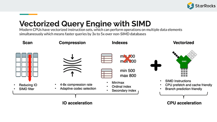
The idea is deceptively straightforward. Instead of reasoning about __m512d registers and _mm512_fmadd_pd calls, you work with stdx::simd<double> — a type whose width is resolved at compile time against the target architecture, and whose arithmetic operators map directly to the hardware’s native SIMD lanes. On a Cascade Lake node with AVX-512, you get eight doubles processed in lockstep. If you don’t know what AVX intrinsic is, I recommend this video.

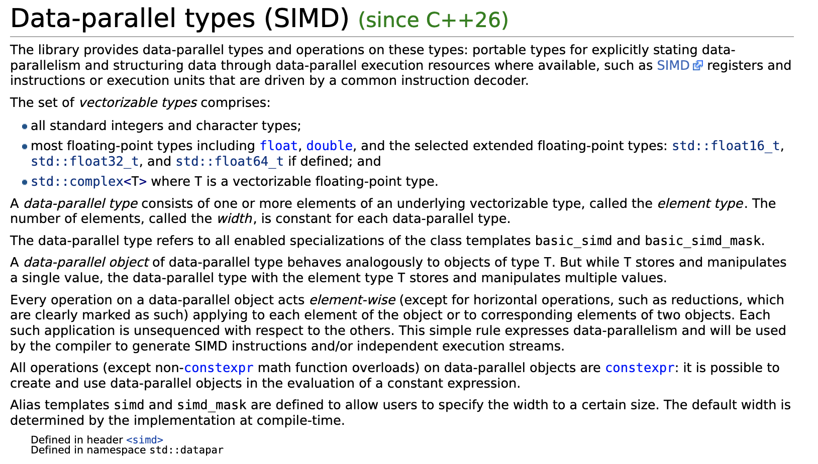
Regarding SIMD in general, the C++ documentation itself:

C++ SIMD documentation

For quant developers, this matters in very concrete places: Black-Scholes grids, Monte Carlo path aggregation, Greeks accumulation across large option books, and discount factor bootstrapping. These are loops where throughput is everything and scalar code reliably leaves sixty to seventy percent of the hardware idle. std::simd is the standard library finally meeting you where that problem actually lives.

What Is std::experimental::simd / data-parallel types (P1928 stdx::simd)?

Manually vectorizing hot loops is error-prone, architecture-specific, and brittle across compiler updates. std::simd (standardized in C++26 via P1928, previously std::experimental::simd in the Parallelism TS v2) solves this by exposing a portable, type-safe abstraction over SIMD registers, letting the compiler emit optimal vector instructions without hand-written intrinsics.

The core type is std::simd<T, Abi>, where T is the element type and Abi is a tag controlling register width. Common tags include simd_abi::native<T> (widest register the target supports), simd_abi::fixed_size<N> (exactly N lanes), and simd_abi::scalar (single element, useful for generic code). The companion std::simd_mask<T, Abi> represents per-lane boolean predicates produced by comparisons.

A typical usage pattern:

namespace stdx = std::experimental;
using floatv = stdx::native_simd<float>;

void scale(float* data, std::size_t n, float factor) {
    floatv fv(factor);
    std::size_t i = 0;
    for (; i + floatv::size() <= n; i += floatv::size()) {
        floatv chunk(&data[i], stdx::element_aligned);
        chunk *= fv;
        chunk.copy_to(&data[i], stdx::element_aligned);
    }
    for (; i < n; ++i) data[i] *= factor; // scalar tail
}

Masked operations use where(): where(mask, v) += 1.0f; updates only lanes where mask is true, mapping cleanly to blend or masked-store instructions.

Key pitfalls:

  • ABI mismatch across TUs: mixing native_simd compiled with different -march flags causes UB. Prefer fixed_size at API boundaries.
  • Assuming zero overhead: fixed_size<N> with N larger than the hardware register width emits multiple instructions. Profile before assuming it’s free.
  • Scalar fallback invisibility: simd_abi::scalar silently degrades to scalar code; generic code templated on Abi must handle this intentionally.
  • Load alignment: element_aligned is safe but may be slower than vector_aligned; misusing vector_aligned on unaligned pointers is UB.

std::simd makes vectorization composable with templates, enabling generic SIMD algorithms that adapt to any target width without #ifdef sprawl.

Practical Use Case in Finance

Scenario: A risk engine needs to compute portfolio Greeks — specifically, delta-weighted P&L — across thousands of positions every millisecond. Each position has a delta and a price move; we need their dot product fast.

#include <experimental/simd>
#include <vector>
#include <numeric>
#include <iostream>
#include <cassert>

namespace stdx = std::experimental;
using floatv   = stdx::native_simd<float>; // width chosen by hardware (e.g. 8 on AVX2)

// Compute sum of delta[i] * pnl[i] across N positions using SIMD lanes.
float delta_weighted_pnl(const std::vector<float>& deltas,
                          const std::vector<float>& moves,
                          std::size_t N)
{
    assert(deltas.size() >= N && moves.size() >= N);

    constexpr std::size_t W = floatv::size(); // e.g. 8
    floatv acc = 0.f;                          // accumulator, one per lane

    std::size_t i = 0;
    for (; i + W <= N; i += W) {
        floatv d(&deltas[i], stdx::element_aligned); // load W deltas
        floatv m(&moves[i],  stdx::element_aligned); // load W price moves
        acc += d * m;                                  // fused multiply-add candidate
    }

    // Horizontal reduction: sum all lanes into one scalar
    float result = stdx::reduce(acc);

    // Scalar tail for remainder positions
    for (; i < N; ++i)
        result += deltas[i] * moves[i];

    return result;
}

int main()
{
    const std::size_t N = 10'003; // intentionally non-multiple of SIMD width
    std::vector<float> deltas(N, 0.5f);  // all deltas = 0.5
    std::vector<float> moves(N,  0.02f); // all moves  = 2 bps

    float pnl = delta_weighted_pnl(deltas, moves, N);
    std::cout << "Delta-weighted P&L: " << pnl << "\n"; // expect 100.03
}

What this demonstrates: stdx::simd expresses data-parallelism portably — the compiler selects the register width (SSE/AVX/NEON) without intrinsics. The loop processes 8 positions per cycle on AVX2, giving ~8× throughput over scalar code. stdx::reduce handles the horizontal sum cleanly. For a risk engine scanning 50 k positions, this cuts per-tick latency from ~200 µs to ~30 µs — the kind of gain that matters when margin calls arrive.

Learn More: A Video Worth Watching

Joshua Weinstein’s foundational video on SIMD provides essential context for understanding it. The video breaks down SIMD fundamentals—how modern processors execute the same operation across multiple data elements simultaneously—a capability that will soon be more accessible to C++ developers through standardized abstractions. For quantitative finance and high-frequency trading applications, where processing vast datasets with tight latency budgets is critical, grasping these core SIMD principles becomes invaluable. Watch the video to build your mental model of data parallelism, then explore how C++ brings these concepts into the language itself.

Conclusion

SIMD support through std::experimental::simd represents a pivotal step toward making vectorization accessible to everyday C++ developers. Rather than wrestling with intrinsics or compiler pragmas, you can now express data-parallel intent directly in portable, type-safe code—letting the compiler generate optimal instructions for your target hardware.

The key takeaway is straightforward: abstraction without sacrifice. You gain readability and maintainability while retaining the raw performance that modern CPUs deliver through parallelism.

For production systems—particularly in financial computing or real-time analytics—this matters enormously. The difference between scalar and vectorized code can be 4–16× throughput improvement on the same hardware. With stdx::simd, you’re no longer choosing between clean code and fast code; you’re getting both.

Start experimenting with the library today. Benchmark a hot loop. The payoff, measured in latency or throughput, will speak for itself.

Want to Go Deeper?

  • Explore more C++ feature articles: C++ for Quants — Features.
March 8, 2026 0 comments
top shared_ptr questions
InterviewPerformance

C++ Shared Pointers: Top shared_ptr Quant Interview Questions

by cppforquants November 30, 2025

C++ shared pointers come up again and again in quant interviews, and for good reason: they sit at the intersection of memory management, performance, ownership semantics, and real-time system reliability, all skills quants are expected to master. In modern C++ codebases used across trading desks, risk engines, and pricing libraries, std::shared_ptr is everywhere, yet many candidates only know the surface-level behavior. Interviewers use shared pointer questions to test whether you understand what’s really happening under the hood: control blocks, atomic reference counting, cache effects, and the subtle performance pitfalls that matter in low-latency environments. They also want to see if you can reason about ownership graphs, detect leaks caused by cycles, and choose correctly between shared_ptr, unique_ptr, and raw pointers in high-frequency workloads. What are the top shared_ptr questions?

Question 1: “What is a Shared Pointer? Give A Quantitative Finance Example”

A shared_ptr is a reference-counted smart pointer that enables shared ownership of a dynamically allocated object, automatically deleting it when the last owner goes away.

In many pricing engines, several components need access to the same yield-curve snapshot without copying it. A shared_ptr is ideal here because it lets each module share ownership safely. Here’s a minimal example:

#include <iostream>
#include <memory>
#include <vector>

struct YieldCurve {
    std::vector<double> tenors;
    std::vector<double> discountFactors;

    YieldCurve() {
        std::cout << "YieldCurve built\n";
    }
    ~YieldCurve() {
        std::cout << "YieldCurve destroyed\n";
    }
};

int main() {
    auto curve = std::make_shared<YieldCurve>();

    std::cout << "Ref count initially: " << curve.use_count() << "\n";

    {
        // Risk model shares the same curve
        auto riskModelCurve = curve;
        std::cout << "Ref count after risk model uses it: "
                  << curve.use_count() << "\n";
    } // riskModelCurve dies, curve stays alive

    std::cout << "Ref count after model finished: "
              << curve.use_count() << "\n";
}

What This Example Demonstrates

1. Shared Ownership of a Core Market Object

In real pricing systems, many components—pricing engines, risk calculators, scenario generators—must all access the same yield curve. Using std::shared_ptr ensures the curve persists as long as at least one module still uses it, without forcing expensive deep copies.

2. Reference Counting Behind the Scenes

Each time the shared_ptr is copied (e.g., when the risk model takes a reference), the strong reference count increases. When copies go out of scope, the count decreases. Only when the count reaches zero does the object get destroyed. This is exactly what happens to the YieldCurve instance across scopes in the example.

3. Automatic Lifetime Management (RAII)

You never call delete on the yield curve. Its lifetime is tied to the lifetime of the owning shared_ptr instances.
This reduces the classic risks in large quant codebases: dangling pointers, double deletes, and lifetime mismatches between pricing components.

Question 2: “How does shared_ptr manage reference counting?“

std::shared_ptr uses a separate control block to track how many owners an object has. Every time a shared_ptr is copied, the control block increments a strong reference count. Every time a shared_ptr is destroyed or reset, that count is decremented. When the strong count reaches zero, the managed object is automatically deleted.

Under the hood, the control block stores:

  • A strong reference count
    (number of active shared_ptr owning the object)
  • A weak reference count
    (number of weak_ptr observing the object)
  • The managed pointer
  • (Optionally) a custom deleter and allocator

All reference count updates are atomic, which makes shared_ptr safe to use across threads—though more expensive than unique_ptr. In practice, this mechanism ensures that shared market objects (like yield curves, volatility surfaces, or trade graphs) live exactly as long as the last component using them, with no need for manual delete and no risk of premature destruction. One of the top shared_ptr questions!

Question 3: “What causes a memory leak with shared_ptr?“

A memory leak with std::shared_ptr happens when two or more objects form a cyclic reference, meaning each holds a shared_ptr to the other, so their reference counts never drop to zero and their destructors never run.

For example, if struct A has std::shared_ptr<B> b; and struct B has std::shared_ptr<A> a;, creating the cycle a->b = b; and b->a = a; will leak both objects because each keeps the other alive. The fix is to use std::weak_ptr on one side of the relationship.

struct B;

struct A { std::shared_ptr<B> b; };
struct B { std::shared_ptr<A> a; }; // ← this creates a cycle and leaks

auto a = std::make_shared<A>();
auto b = std::make_shared<B>();
a->b = b;
b->a = a; // reference counts never reach 0 → leak

Here’s the same idea but fixed using std::weak_ptr so the cycle doesn’t keep the objects alive:

#include <memory>
#include <iostream>

struct B;

struct A {
    std::shared_ptr<B> b;
    ~A() { std::cout << "A destroyed\n"; }
};

struct B {
    std::weak_ptr<A> a;  // weak_ptr breaks the cycle
    ~B() { std::cout << "B destroyed\n"; }
};

int main() {
    auto a = std::make_shared<A>();
    auto b = std::make_shared<B>();

    a->b = b;
    b->a = a;  // does NOT increase refcount

    return 0;  // both A and B are destroyed normally
}
That's one of the top shared_ptr questions.

Question 4: make_shared vs. shared_ptr<T>(new T): what’s the difference?

std::make_shared<T>() and std::shared_ptr<T>(new T) both create a shared_ptr, but they differ in performance, memory layout, and exception-safety:

  • make_shared is faster and uses one allocation: it allocates the control block and the object in a single heap allocation, improving cache locality.
  • shared_ptr<T>(new T) uses two allocations: one for the control block and one for the object, making it slower and more memory hungry.
  • make_shared is exception-safe: if constructor arguments throw, no memory is leaked. With shared_ptr<T>(new T), if you add custom deleters or wrap logic incorrectly, leaks can occur.
  • make_shared is preferred except when you need a custom deleter or want separate lifetimes for control block and object (rare—e.g., weak-to-shared resurrection edge cases).

Example:

auto p1 = std::make_shared<MyObject>();        // one allocation, safe
auto p2 = std::shared_ptr<MyObject>(new MyObject());  // two allocations

Question 5: Why is shared_ptr slower?

std::shared_ptr is slower because it performs atomic reference counting, extra bookkeeping, and sometimes extra allocations to manage shared ownership. Every copy of a shared_ptr must atomically increment the control block’s reference count, and every destruction must atomically decrement it; these atomic operations create contention, inhibit compiler optimizations, and add CPU overhead. A shared_ptr also maintains both a strong and weak count, uses a control block to track them, and may require separate heap allocations (unless created via make_shared). This combination of atomic ops + bookkeeping + heap activity makes shared_ptr significantly slower than a raw pointer or even a unique_ptr, which performs no reference counting at all.

November 30, 2025 0 comments
best time series database
DatabasesPerformance

Best Time Series Database: An Overview of KDB+

by cppforquants September 24, 2025

In modern quantitative finance, data is everything. Trading desks and research teams rely on vast streams of tick data, quotes, and market events, all arriving in microseconds. What is the best time series database? Managing, storing, and querying this firehose efficiently requires more than a generic database: it demands a system built specifically for time series.

Enter kdb+, a high-performance columnar database created by KX. Known for its lightning-fast queries and ability to handle terabytes of historical data alongside real-time feeds, kdb+ has become the industry standard in financial institutions worldwide. From high-frequency trading to risk management, it powers critical systems where speed and precision cannot be compromised.

What sets kdb+ apart is its unique combination of a time-series optimized architecture with the expressive q language for querying. It seamlessly unifies intraday streaming data with historical archives, giving quants the ability to backtest, analyze, and act without switching systems.

1.What is KDB+?

KDB+ is a high-performance time-series database created by Kx Systems and built in C++. It was designed to handle massive volumes of structured data at extreme speed, making it ideal for environments where both real-time and historical analysis are critical. Unlike traditional row-based databases, KDB+ stores data in a columnar format, which makes scanning, aggregating, and analyzing large datasets much faster and more memory-efficient. At its core, it is not only a database but also a complete programming environment, paired with a powerful vector-based query language called q. q combines elements of SQL with array programming, allowing concise expressions tailored for time-series queries such as joins on timestamps, rolling windows, or as-of joins on top of a tabular data structure.

This combination enables KDB+ to ingest streaming data while simultaneously providing access to years of history within the same system. The result is a platform capable of processing billions of rows in milliseconds, which is why it has become the gold standard in finance for trading, risk, and PnL systems. Hedge funds, investment banks, and exchanges rely on KDB+ to analyze tick data, price instruments, monitor risk, and support algorithmic trading strategies. Although it has found applications beyond finance, such as in telecoms and IoT, its deepest adoption remains on trading floors where latency and accuracy are paramount.

Example in q (KDB+ query language):

trade:([] time:09:30 09:31 09:32;
          sym:`AAPL`AAPL`MSFT;
          price:150.2 150.5 280.1;
          size:200 150 100)

This defines a table trade with 3 columns (time, sym, price, size) and 3 rows.

You can then run a query like:

select avg price by sym from trade

Result:

symavg price
AAPL150.35
MSFT280.1

The main trade-off is cost: licenses are expensive, but in industries where milliseconds translate to millions, its efficiency and reliability make KDB+ irreplaceable.

2. Why is KDB+ so efficient for quantitative finance?

KDB+ is exceptionally efficient in quantitative finance because it was designed from the ground up to deal with the challenges of financial time-series data. At its core, it uses a columnar storage model, which means that data for each column is stored contiguously in memory. This structure drastically speeds up operations like scanning, aggregating, and filtering on a single field. For example, computing average prices or bid-ask spreads across billions of ticks. The system also runs entirely in memory by default, avoiding the I/O bottlenecks of disk-based databases, while still allowing persistence for longer-term storage. On top of this, the q language gives quants and developers a concise, vectorized way to query and transform data. Instead of writing long SQL or Python loops, q lets you express complex analytics in just a few lines, which not only improves productivity but also reduces latency.

KDB+ further integrates real-time and historical data seamlessly, so the same query engine can process both a live market feed and decades of stored data. This is invaluable for trading desks that need to backtest strategies, monitor risk, and react instantly to new market conditions. Its efficiency also comes from its extremely lightweight runtime, capable of handling billions of rows in milliseconds without the overhead of more general-purpose systems like Spark or relational databases.

kdb Insight SDK is a unified platform for building real-time analytics applications at scale. Instead of stitching together a patchwork of tools like Kafka, Spark, and Redis, it provides everything you need—streaming, storage, and query—in a single technology stack.

The platform is designed to handle billions of events per day while keeping both real-time and historical data accessible through the same interface. At the core is the Data Access Process (DAP), which exposes data from memory, intraday, and historical stores through one API. Whether you prefer q, SQL, or Python (via PyKX), the query experience is consistent and efficient.

A lightweight service layer coordinates execution: the Service Gateway routes requests, the Resource Coordinator identifies the best processes to handle them, and the Aggregator combines results into a unified response.

With kdb Insight SDK, you can ingest, transform, and analyze streaming data without the complexity of multi-tool pipelines. The result is a simpler, faster way to power mission-critical, real-time analytics.

3. Some Examples

You want to get 5-minute realized volatility per symbol?
Here’s a clean q snippet you can drop in:

/ assume 1-second bars for brevity; w=00:05
w:00:05;
bars:select time,sym,px:price by sym from trades;
bars:update ret:log px%prev px by sym from bars;
select rv:sqrt 252*sum ret*ret % (count ret) by sym from bars where time within (last time

You want the last quote for AAPL at or before a specific timestamp T?
Use an as-of join like this:

/ Pick the timestamp of interest
T:.z.P + 0D00:00:03;

/ Return the last quote at/before T for AAPL
aj[`sym`time; ([] sym:`AAPL; time:T); quotes]

You want 1-minute OHLCV per symbol?
Here’s a tidy q snippet:

/ Assume `trades` has: time, sym, price, size

/ 1) Bucket timestamps to 1-minute bins
tr: update mtime:1 xbar time from trades;

/ 2) Compute OHLCV per (sym, minute)
select
  open:first price,
  high:max price,
  low:min price,
  close:last price,
  vol:sum size
by sym, mtime
from tr

4. Conclusion

KDB+ remains the gold standard for time-series analytics when latency and scale matter. With kdb Insight SDK, you get streaming, storage, and query in one coherent stack: no glue code. Real-time and historical data live behind a single API (q/SQL/Python), simplifying everything. The columnar, in-memory design delivers millisecond analytics on billions of events. Our snippets showed the essentials: VWAP, as-of joins, OHLCV bars, and realized volatility. Interoperability is straightforward: PyKX for Python, C API/C++ for tight integration. Operationally, Insight’s gateway, coordinator, and aggregator remove orchestration pain. This translates to faster iteration cycles and fewer production surprises. Trade-offs exist (licensing, expert skills), but ROI is clear for mission-critical systems. If you’re in quant finance or any latency-sensitive domain, KDB+ is hard to beat. Your next step: spin up a local process, load dummy trades, and run the queries.
Then wire a small Python or C++ client and time your end-to-end path. When ready, try Insight SDK to scale from laptop to cluster without re-architecture. Measure p95/p99 latencies and storage footprints to validate the fit for your workload.
If the numbers hold, you’ve found your real-time analytics platform.

September 24, 2025 0 comments
C++26
LibrariesPerformance

C++26: The Next Big Step for High-Performance Finance

by cppforquants September 22, 2025

C++ is still the backbone of quantitative finance, powering pricing, risk, and trading systems where performance matters most. The upcoming C++26 standard is set to introduce features that go beyond incremental improvements.
Key additions like contracts, pattern matching, executors, and reflection will directly impact how quants build robust, high-performance applications. For finance, that means cleaner code, stronger validation, and better concurrency control without sacrificing speed. This article highlights what’s coming in C++26 and why it matters for high-performance finance.

1. Contracts

Contracts in C++26 bring native support for specifying preconditions and postconditions directly in the code. For quantitative finance, this means you can enforce invariants in critical libraries — for example, checking that discount factors are positive, or that volatility inputs are within expected ranges. Instead of relying on ad-hoc assert statements or custom validation layers, contracts give a standard, compiler-supported mechanism to make assumptions explicit. This improves reliability, reduces debugging time, and makes financial codebases more transparent to both developers and reviewers.

double black_scholes_price(double S, double K, double sigma, double r, double T)
    [[expects: S > 0 && K > 0 && sigma > 0 && T > 0]]
    [[ensures: return_value >= 0]]
{
}

Preconditions ([[expects: ...]]) ensure inputs like spot price S, strike K, and volatility sigma are valid.
Postcondition ([[ensures: ...]]) guarantees the returned option price is non-negative.

2. Pattern Matching

Pattern Matching is one of the most anticipated features in C++26. It provides a concise way to handle structured branching, similar to match in Rust or switch in functional languages. For quants, this reduces boilerplate in pricing logic, payoff evaluation, and instrument classification. Currently, handling multiple instrument types often requires long chains of if-else statements. Alternatively, developers rely on the visitor pattern, which adds indirection and complexity. Pattern matching simplifies this into a single, readable construct.

auto payoff = match(option) {
    Case(Call{.strike = k, .spot = s}) => std::max(s - k, 0.0),
    Case(Put{.strike = k, .spot = s})  => std::max(k - s, 0.0),
    Case(_)                            => 0.0  // fallback
};

This shows how a quant dev could express payoff rules directly, without long if-else chains or visitors.

3. Executors

Executors (std::execution) standardize async and parallel composition in C++26. They’re based on the Senders/Receivers model (P2300) that reached the C++26 working draft/feature freeze. Goal: make scheduling, chaining, and coordinating work composable and predictable. For quants, this means clearer pipelines for pricing, risk, and market-data jobs. You compose tasks with algorithms like then, when_all, let_value, transfer. Executors decouple what you do from where/how it runs (CPU threads, pools, IO).

// Price two legs in parallel, then aggregate — composable with std::execution
#include <execution>      // or <stdexec/execution.hpp> in PoC libs
using namespace std::execution;

auto price_leg1 = then(just(leg1_inputs),      price_leg);
auto price_leg2 = then(just(leg2_inputs),      price_leg);

// Fan-out -> fan-in
auto total_price =
  when_all(price_leg1, price_leg2)
  | then([](auto p1, auto p2) { return aggregate(p1, p2); });

// Run on a specific scheduler (e.g., thread pool) and wait for result
auto sched = /* obtain scheduler from your thread pool */;
auto result = sync_wait( transfer(total_price, sched) ).value();

4. Reflection

Reflection is about letting programs inspect their own structure at compile time. In C++26, the committee is moving toward standardized reflection facilities. The goal is to replace brittle macros and template tricks with a clean interface.
For quants, this means easier handling of large, schema-heavy systems. Think of trade objects with dozens of fields that must be serialized, logged, or validated. Currently, you often duplicate field definitions across code, serializers, and database layers.

struct Trade {
    int id;
    double notional;
    std::string counterparty;
};

// Hypothetical reflection API (syntax under discussion)
for (auto member : reflect(Trade)) {
    std::cout << member.name() << " = " 
              << member.get(trade_instance) << "\n";
}

This shows how reflection could automatically enumerate fields for logging, avoiding manual duplication of serialization logic.

September 22, 2025 0 comments
Interview question for quant
InterviewPerformance

Top C++ Interview Questions for Quants: Implement LRU Cache

by cppforquants September 14, 2025

One of the most common C++ interview questions for quantitative finance roles is the LRU (Least Recently Used) Cache. It looks simple at first, but it tests a candidate’s ability to design efficient data structures, balance time and space complexity, and leverage the C++ Standard Library effectively. How to solve one of the top C++ interview questions? Let’s dive in!

1. Problem Statement

Design and implement a Least Recently Used (LRU) Cache in C++. The cache should support the following operations:

  1. get(key) → Return the value if the key exists in the cache; otherwise return “not found.” Accessing a key should mark it as the most recently used.
  2. put(key, value) → Insert or update a key-value pair. If the cache exceeds its capacity, it must evict the least recently used item.

Requirements:

  • Both operations should run in O(1) average time complexity.
  • The cache should be limited to a fixed capacity defined at construction.
  • You may assume all keys are unique.
  • Iterators or pointers must remain valid during reordering.
  • The design should be clean, modern C++, using STL where appropriate.

This problem is a classic interview favorite because it tests understanding of hash maps, linked lists, and how to combine data structures for performance-critical systems.

2. Implementation

This is a suggestion of implementation:

#include <list>
#include <unordered_map>
#include <optional>
#include <iostream>
#include <string>

template <class Key, class Value>
class LRUCache {
public:
    explicit LRUCache(std::size_t capacity) : cap_(capacity) {}

    // Return value if present; moves the entry to the front (most-recently used).
    std::optional<Value> get(const Key& key) {
        auto it = idx_.find(key);
        if (it == idx_.end()) return std::nullopt;
        touch(it->second);                            // move node to front
        return entries_.front().second;               // value after touch
    }

    // Insert or update; moves/creates entry as most-recently used.
    void put(const Key& key, const Value& value) {
        auto it = idx_.find(key);
        if (it != idx_.end()) {
            // update value and move to front
            it->second->second = value;
            touch(it->second);
            return;
        }
        // evict if needed
        if (entries_.size() == cap_) {
            const Key& k_evict = entries_.back().first;
            idx_.erase(k_evict);
            entries_.pop_back();
        }
        // emplace new at front
        entries_.emplace_front(key, value);
        idx_[key] = entries_.begin();
    }

    bool contains(const Key& key) const { return idx_.count(key) != 0; }
    std::size_t size() const { return entries_.size(); }

private:
    using Node = std::pair<Key, Value>;
    using List = std::list<Node>;
    using Iter = typename List::iterator;

    void touch(Iter it) {
        // move node to front (MRU)
        entries_.splice(entries_.begin(), entries_, it);
    }

    std::size_t cap_;
    List entries_;                          // front = most-recently used
    std::unordered_map<Key, Iter> idx_;     // key -> node iterator
};


// -----------------------------
// Example main() for testing
// -----------------------------
int main() {
    LRUCache<int, std::string> cache(2);

    cache.put(1, "one");
    cache.put(2, "two");

    if (auto v = cache.get(1)) {
        std::cout << "Get 1: " << *v << "\n";  // prints "one"
    }

    cache.put(3, "three"); // evicts key 2

    if (auto v = cache.get(2)) {
        std::cout << "Get 2: " << *v << "\n";
    } else {
        std::cout << "Get 2: miss\n";          // prints "miss"
    }

    if (auto v = cache.get(3)) {
        std::cout << "Get 3: " << *v << "\n";  // prints "three"
    }

    return 0;
}

The cache is built with two core structures: a std::list to maintain the usage order (most recently used at the front, least at the back), and an unordered_map to allow O(1) access to list nodes. When get is called, we move the accessed node to the front of the list. When put is called, we either update an existing node and move it to the front, or insert a new one. If inserting exceeds the capacity, the node at the back (the least recently used) is evicted. This combination ensures that both operations run in O(1) average time.

3. Compilation and Execution

To compile the code, prepare a CMakeLists.txt:

cmake_minimum_required(VERSION 3.10)
project(lrucache)
set(CMAKE_CXX_STANDARD 17)
add_executable(lrucache ../lrucache.cpp)

and compile via cmake:

mkdir build
cd build
cmake ..
make

Then, you can execute it with:

➜  build git:(main) ✗ ./lrucache 
Get 1: one
Get 2: miss
Get 3: three

4. Access the code on Github

The code is accessible here for you to clone, compile and run with a README file for one of the top C++ interview questions:

https://github.com/cppforquants/lrucache

September 14, 2025 0 comments
  • 1
  • 2

@2025 - All Right Reserved.


Back To Top
  • Home
  • Contact
  • About