Commodity Forwards in C++: A Quantlib Implementation

Commodity forwards are among the simplest derivatives conceptually: two counterparties agree today on a price for a commodity that will be delivered or settled at a future date. The contract itself is straightforward, but valuing an existing forward requires understanding the distinction between the price written into the contract and the current market forward price for the same delivery. How to value commodity forwards in C++?

In this article, we build a simple commodity-forward valuation workflow in C++ using QuantLib. We start from a set of market quotes across several delivery dates, construct an interpolated forward curve, retrieve the current forward price for a specific maturity, discount the resulting payoff, and calculate the mark-to-market value of an existing contract.

1. Commodity Forward Contracts

A commodity forward is an agreement between two counterparties to buy or sell a specified quantity of a commodity at a predetermined price on a future delivery date.

Consider a crude-oil forward entered into in September with the following terms:

Commodity: crude oil
Position: long
Quantity: 1,000 barrels
Delivery: December 2026
Forward price: $69 per barrel

The contractual delivery price is therefore: $K = \$69$

and the quantity is: $Q=1,000.$

In December, the long counterparty is contractually entitled to buy 1,000 barrels for $69 per barrel, regardless of how the market price of crude oil has changed.

When the forward is initially entered into, its contractual price is normally chosen so that the contract has approximately zero value:
$K=F_0(T)$

where $F_0(T)$ is the market forward price for delivery at $T$ .

Therefore: $V_0=0.$

This is an important distinction: the forward price and the value of a forward contract are not the same thing.

2. Valuing Existing Commodity Forwards in C++: The Theory

For a simple commodity forward, its value to the long can be written as:

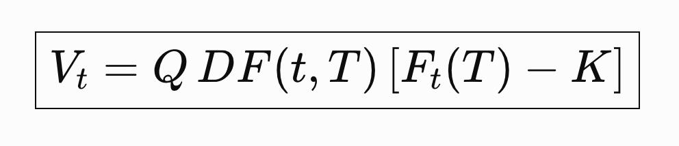
where:

$Q$ is the quantity of commodity,
$K$ is the contractual forward price,
$F_t(T)$ is today’s market forward price for delivery at $T$ ,
$DF(t,T)$ is the discount factor between today and delivery.

Suppose: $Q=1,000$ $K=69$ $F_t(T)=72$

and: $DF(t,T)=0.99.$

The value is: Vt=1,000×0.99×(72−69)=$2,970

The forward therefore has a positive value of approximately $2,970 to the long counterparty.

3. The Commodity Forward Curve

The remaining question is where:
$F_t(T)$

comes from.

Commodity markets trade instruments corresponding to different future delivery periods. A simplified set of observable crude-oil market prices might look like:

Delivery	Market Price
October 2026	$71.20
November 2026	$70.80
December 2026	$70.10
January 2027	$69.60

These points describe the current shape of the commodity market across different maturities:
$(T_1,F_1),\;(T_2,F_2),\ldots,(T_n,F_n).$
Collectively, they form a discrete representation of the commodity forward curve.

For exchange-traded commodities, some of the most directly observable prices will actually be futures prices rather than OTC forward quotes.

Futures and forwards provide closely related economic exposure, but they are not identical instruments. Futures are standardized, exchange-cleared contracts whose gains and losses are settled through daily variation margin. Forwards are bilateral OTC contracts whose terms can be customized.

Under simplifying assumptions, futures prices can nevertheless provide useful market inputs for constructing the curve used to mark an OTC forward.

4. Representing the Market Curve with QuantLib

A first step to value commodity forwards in C++ is to represent our market data using QuantLib dates and prices:

#include <ql/quantlib.hpp>

#include <iostream>
#include <vector>

using namespace QuantLib;

int main()
{
    Date today(13, September, 2026);
    Settings::instance().evaluationDate() = today;

    std::vector<Date> deliveryDates = {
        Date(1, October, 2026),
        Date(1, November, 2026),
        Date(1, December, 2026),
        Date(1, January, 2027)
    };

    std::vector<Real> futuresPrices = {
        71.20,
        70.80,
        70.10,
        69.60
    };
}

At this point we have discrete market observations but not yet a continuous curve.

For example, we know the market prices corresponding to November 1 and December 1, but not necessarily the price corresponding to a delivery date such as November 15.

We therefore need interpolation.

5. From the Forward Curve to the Forward Value

Once the market quotes have been converted into a forward curve, valuing the contract is straightforward.

QuantLib’s LinearInterpolation allows us to estimate $F_t(T)$ for a delivery date that falls between the quoted market maturities. For example, if our delivery date lies between the November and December contracts, the interpolated value provides an estimate of the current market forward price for that date. We then compare this value with the contractual price $K$ agreed when the forward was entered into. Because this difference represents value associated with a future settlement date, it must be discounted back to today. For simplicity, we use a flat 4% QuantLib FlatForward interest-rate curve to obtain the discount factor $DF(t,T)$ ; in a production system, this would normally be replaced by an appropriately constructed market discount curve. The value of the forward to the long is therefore given by the formula given in 2.

A positive value means the contract is valuable to the long because it allows the commodity to be purchased below the current market forward price; the value to the short is the opposite. The complete C++ implementation below performs this entire sequence: market quotes → interpolation → current forward price → discount factor → NPV.

6. Complete C++ Example

So, how to price commodity forwards in C++?

#include <ql/quantlib.hpp>

#include <iostream>
#include <vector>

using namespace QuantLib;

Real valueCommodityForward(
    Real quantity,
    Real strike,
    const Date& delivery,
    const LinearInterpolation& forwardCurve,
    const YieldTermStructure& discountCurve,
    const Date& today,
    const DayCounter& dayCounter)
{
    Time t =
        dayCounter.yearFraction(today, delivery);

    Real marketForward =
        forwardCurve(t);

    DiscountFactor df =
        discountCurve.discount(delivery);

    return quantity
         * (marketForward - strike)
         * df;
}

int main()
{
    Date today(13, September, 2026);
    Settings::instance().evaluationDate() = today;

    Actual365Fixed dayCounter;

    std::vector<Date> deliveryDates = {
        Date(1, October, 2026),
        Date(1, November, 2026),
        Date(1, December, 2026),
        Date(1, January, 2027)
    };

    std::vector<Real> futuresPrices = {
        71.20,
        70.80,
        70.10,
        69.60
    };

    std::vector<Time> times;

    for (const auto& date : deliveryDates) {
        times.push_back(
            dayCounter.yearFraction(today, date)
        );
    }

    LinearInterpolation forwardCurve(
        times.begin(),
        times.end(),
        futuresPrices.begin()
    );

    Handle<YieldTermStructure> discountCurve(
        ext::make_shared<FlatForward>(
            today,
            0.04,
            dayCounter
        )
    );

    Real quantity = 1000.0;
    Real strike = 69.0;

    Date delivery(15, November, 2026);

    Real npv = valueCommodityForward(
        quantity,
        strike,
        delivery,
        forwardCurve,
        *discountCurve,
        today,
        dayCounter
    );

    std::cout
        << "Commodity forward NPV: $"
        << npv
        << '\n';

    return 0;
}

First, we define today’s date and provide a small set of commodity market prices for different future delivery dates. Because the market only gives us prices at specific maturities, we use QuantLib’s LinearInterpolation to construct a simple forward curve and estimate $F_t(T)$ for our exact delivery date.

We then create a simple interest-rate curve using QuantLib’s FlatForward with a 4% rate. This gives us the discount factor needed to convert the future value of the contract into today’s value.

Finally, the valueCommodityForward function brings everything together. It retrieves the interpolated market forward price, obtains the discount factor, and calculates the value of the forward based on the formula from the former section.