
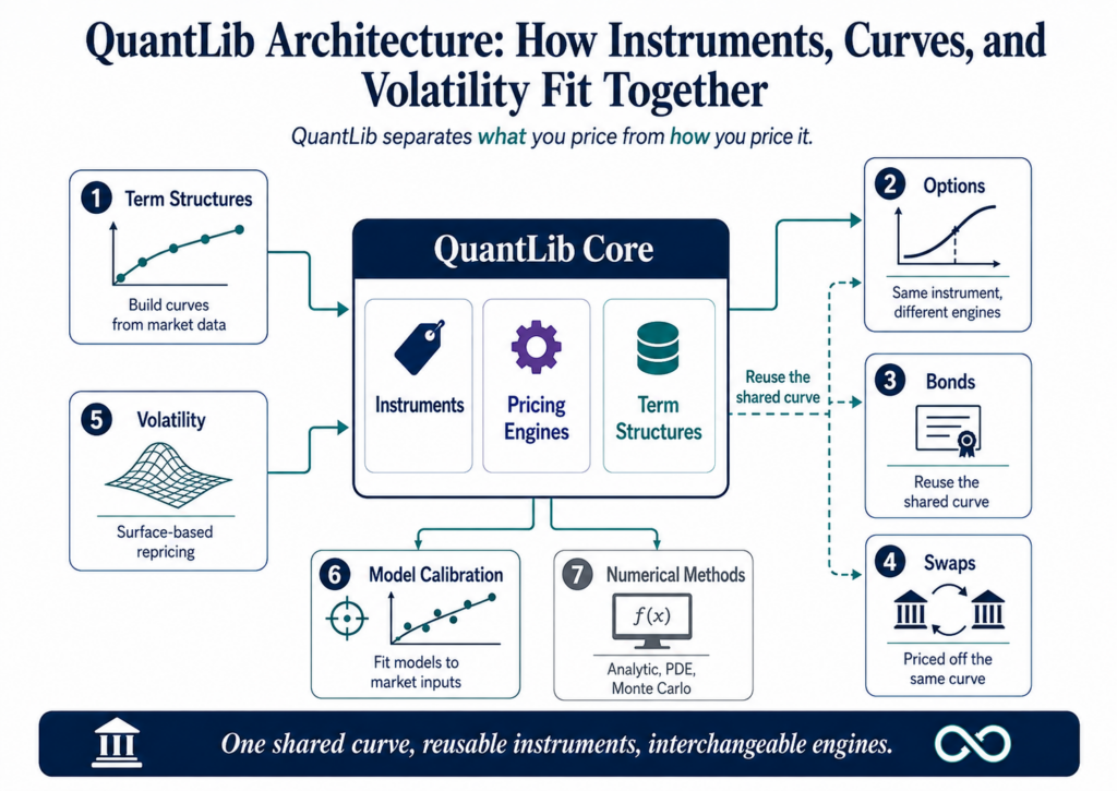
The QuantLib architecture is designed around a clear separation between financial instruments, market data, models, and pricing engines. Instead of tightly coupling each product to a single valuation method, QuantLib lets developers reuse shared term structures, volatility surfaces, and market inputs across options, bonds, swaps, and other instruments.
This modular design is one of the main reasons QuantLib is widely used for quantitative finance and derivatives pricing. In this article, we’ll explore how the core pieces of the QuantLib architecture fit together: from yield curves and volatility structures to pricing engines, numerical methods, and model calibration, and how the same market infrastructure can support multiple valuation workflows.
1. Term Structures
A term structure describes how a financial quantity changes with maturity. In the case of a yield/discount curve, it answers questions such as:
- What is the discount factor for a cash flow occurring in 3 months?
- What is the implied zero rate for 5 years?
- What is the forward rate between years 5 and 7?
The important idea in QuantLib is that a curve is not simply an array of rates. Market data usually gives you only a finite set of quotes—for example, a 3-month deposit rate and swap rates at 1Y, 2Y, 5Y, 10Y, etc. Pricing, however, may require a value at any date.
QuantLib therefore represents the curve as a queryable object. You provide the market instruments and their quotes, and the bootstrapping machinery constructs a YieldTermStructure. You can then ask that object for discount factors, zero rates, or forward rates at arbitrary dates. Interpolation and the conventions used to construct the curve are encapsulated by the term structure rather than being left to every pricing model.
A useful mental model is in the Quantlib architecture framework:
Market quotes → calibration/bootstrapping → queryable term structure → pricing
For example, a discount curve might be bootstrapped from a short-dated deposit followed by a set of interest-rate swaps:
#include <ql/quantlib.hpp>

using namespace QuantLib;

int main() {
    Calendar calendar = TARGET();
    Date today = Date(9, August, 2026);
    Settings::instance().evaluationDate() = today;

    DayCounter dc = Actual365Fixed();

    // Market quotes
    auto depositRate =
        ext::make_shared<SimpleQuote>(0.0250);

    auto swapRate1Y =
        ext::make_shared<SimpleQuote>(0.0270);

    auto swapRate5Y =
        ext::make_shared<SimpleQuote>(0.0320);

    auto swapRate10Y =
        ext::make_shared<SimpleQuote>(0.0350);

    // Convert quotes into RateHelpers.
    auto deposit = ext::make_shared<DepositRateHelper>(
        Handle<Quote>(depositRate),
        Period(3, Months),
        2,
        calendar,
        ModifiedFollowing,
        false,
        Actual360()
    );

    auto swap1Y = ext::make_shared<SwapRateHelper>(
        Handle<Quote>(swapRate1Y),
        Period(1, Years),
        calendar,
        Annual,
        Unadjusted,
        Thirty360(Thirty360::BondBasis),
        Euribor6M()
    );

    auto swap5Y = ext::make_shared<SwapRateHelper>(
        Handle<Quote>(swapRate5Y),
        Period(5, Years),
        calendar,
        Annual,
        Unadjusted,
        Thirty360(Thirty360::BondBasis),
        Euribor6M()
    );

    auto swap10Y = ext::make_shared<SwapRateHelper>(
        Handle<Quote>(swapRate10Y),
        Period(10, Years),
        calendar,
        Annual,
        Unadjusted,
        Thirty360(Thirty360::BondBasis),
        Euribor6M()
    );

    std::vector<ext::shared_ptr<RateHelper>> helpers = {
        deposit, swap1Y, swap5Y, swap10Y
    };

    // Bootstrap the curve from the market instruments.
    auto curve = ext::make_shared<PiecewiseYieldCurve<Discount, LogLinear>>(
        today,
        helpers,
        dc
    );

    // The curve is queryable at arbitrary dates.
    Date fiveYears = calendar.advance(today, Period(5, Years));

    Real discountFactor = curve->discount(fiveYears);
    Rate zeroRate = curve->zeroRate(fiveYears, dc, Continuous).rate();

    std::cout << "5Y discount factor: " << discountFactor << '\n';
    std::cout << "5Y zero rate:       " << zeroRate << '\n';
}
2. Options Pricing
Options pricing is a big big deal in quantitative finance.
In the QuantLib architecture, an Instrument represents the financial contract: its payoff, exercise rules, maturity, and other contractual properties. It does not need to know how its value will be calculated.
The actual valuation is delegated to a PricingEngine.
That separation is useful because the same option can be priced using different numerical methods without changing the definition of the option itself. For example, a European vanilla option can be valued with an analytic Black–Scholes engine, or with a Monte Carlo engine. The VanillaOption remains the same; only the pricing engine changes.
A useful mental model is:
Market data + Instrument → PricingEngine → valuation
Or, more specifically:
What are we pricing? →
VanillaOption
How are we pricing it? →PricingEngine
Here’s a simple European call:
#include <ql/quantlib.hpp>

using namespace QuantLib;

int main() {
    Date today(9, August, 2026);
    Settings::instance().evaluationDate() = today;

    Calendar calendar = TARGET();
    DayCounter dc = Actual365Fixed();

    // Market inputs
    Handle<Quote> spot(
        ext::make_shared<SimpleQuote>(100.0)
    );

    Handle<YieldTermStructure> riskFreeCurve(
        ext::make_shared<FlatForward>(
            today, 0.03, dc
        )
    );

    Handle<YieldTermStructure> dividendCurve(
        ext::make_shared<FlatForward>(
            today, 0.00, dc
        )
    );

    Handle<BlackVolTermStructure> volatility(
        ext::make_shared<BlackConstantVol>(
            today, calendar, 0.20, dc
        )
    );

    // Define the option contract.
    auto payoff = ext::make_shared<PlainVanillaPayoff>(
        Option::Call,
        100.0
    );

    Date maturity = calendar.advance(
        today, Period(1, Years)
    );

    auto exercise = ext::make_shared<EuropeanExercise>(
        maturity
    );

    VanillaOption option(payoff, exercise);

    // Choose how to price it.
    auto engine = ext::make_shared<AnalyticEuropeanEngine>(
        Handle<GeneralizedBlackScholesProcess>(
            ext::make_shared<GeneralizedBlackScholesProcess>(
                spot,
                dividendCurve,
                riskFreeCurve,
                volatility
            )
        )
    );

    option.setPricingEngine(engine);

    std::cout << "Option value: "
              << option.NPV()
              << '\n';
}
3. Bonds Pricing
A bond is a sequence of future cash flows: coupons and, eventually, repayment of principal. To value the bond today, those future cash flows need to be discounted back to the valuation date.
In the QuantLib architecture, the FixedRateBond represents the bond contract and its cash flows. It doesn’t itself contain the logic for discounting those cash flows.
The DiscountingBondEngine provides that valuation logic. It takes a YieldTermStructure—such as the curve bootstrapped in the previous section—and uses its discount factors to calculate the present value of the bond’s future cash flows.
So the architecture becomes:
Market quotes → YieldTermStructure → PricingEngine → Instrument value
And importantly, the same curve can be shared by many instruments:
One curve → bonds, swaps, options, and other instruments
Here’s a simple fixed-rate bond using a discount curve:
#include <ql/quantlib.hpp>

using namespace QuantLib;

int main() {
    Date today(9, August, 2026);
    Settings::instance().evaluationDate() = today;

    Calendar calendar = TARGET();
    DayCounter dc = ActualActual(ActualActual::Bond);

    // In practice, this would be the bootstrapped curve
    // from Section 1.
    Handle<YieldTermStructure> discountCurve(
        ext::make_shared<FlatForward>(
            today,
            0.03,
            dc
        )
    );

    // Define the bond.
    Natural settlementDays = 2;
    Date issueDate = today;
    Date maturityDate = calendar.advance(
        issueDate, Period(5, Years)
    );

    Schedule schedule(
        issueDate,
        maturityDate,
        Period(Annual),
        calendar,
        Unadjusted,
        Unadjusted,
        DateGeneration::Backward,
        false
    );

    Real couponRate = 0.04;

    FixedRateBond bond(
        settlementDays,
        100.0,                  // face value
        schedule,
        std::vector<Rate>{couponRate},
        dc
    );

    // Tell the bond how it should be valued.
    auto engine =
        ext::make_shared<DiscountingBondEngine>(
            discountCurve
        );

    bond.setPricingEngine(engine);

    std::cout << "Bond NPV: "
              << bond.NPV()
              << '\n';

    std::cout << "Clean price: "
              << bond.cleanPrice()
              << '\n';

    std::cout << "Dirty price: "
              << bond.dirtyPrice()
              << '\n';
}
Another example in this video:
4. Interest Rate Swaps
An interest rate swap exchanges two streams of interest payments, typically a fixed rate against a floating rate. In a vanilla fixed-for-floating swap, one party pays a fixed rate while receiving a floating rate, usually based on an index such as 6-month Euribor.
From a pricing perspective, the swap is essentially a comparison of two legs:
- the fixed leg, whose future payments are known from the swap’s fixed rate;
- the floating leg, whose future payments depend on the evolution of interest rates.
QuantLib architecture represents the contract with VanillaSwap. The actual valuation is delegated to a pricing engine, such as DiscountingSwapEngine.
This is where the term structure from Section 1 becomes particularly useful. The same YieldTermStructure that was bootstrapped from market quotes can be passed into the swap’s pricing engine to discount the swap’s future cash flows.
A useful mental model is:
Curve → discounting and forward-rate information → swap valuation
Or, across the sections you’ve built so far:
Market quotes → YieldTermStructure → financial instrument → PricingEngine → NPV
Here is a simple vanilla swap:
#include <ql/quantlib.hpp>

using namespace QuantLib;

int main() {
    Date today(9, August, 2026);
    Settings::instance().evaluationDate() = today;

    Calendar calendar = TARGET();
    DayCounter dc = Actual365Fixed();

    // In practice, reuse the bootstrapped curve
    // from Section 1.
    Handle<YieldTermStructure> curve(
        ext::make_shared<FlatForward>(
            today,
            0.03,
            dc
        )
    );

    // Swap terms
    Date startDate = calendar.advance(
        today, Period(2, Days)
    );

    Date maturityDate = calendar.advance(
        startDate, Period(5, Years)
    );

    Schedule fixedSchedule(
        startDate,
        maturityDate,
        Period(Annual),
        calendar,
        ModifiedFollowing,
        ModifiedFollowing,
        DateGeneration::Forward,
        false
    );

    Schedule floatingSchedule(
        startDate,
        maturityDate,
        Period(Semiannual),
        calendar,
        ModifiedFollowing,
        ModifiedFollowing,
        DateGeneration::Forward,
        false
    );

    // Build the vanilla fixed-for-floating swap.
    Rate fixedRate = 0.0325;

    VanillaSwap swap(
        VanillaSwap::Payer,       // pay fixed, receive floating
        1'000'000.0,              // notional
        fixedSchedule,
        fixedRate,
        dc,
        floatingSchedule,
        Euribor6M(curve),
        0.0,                       // spread
        Actual360()
    );

    // Use the same curve to discount the swap.
    auto engine =
        ext::make_shared<DiscountingSwapEngine>(curve);

    swap.setPricingEngine(engine);

    std::cout << "Swap NPV: "
              << swap.NPV()
              << '\n';

    std::cout << "Fair fixed rate: "
              << swap.fairRate()
              << '\n';
}
5. Volatility Surface
A volatility surface captures this two-dimensional relationship and it can often look like a smile.
In QuantLib architecture, BlackVarianceSurface represents this market information as a queryable object. Instead of asking for “the volatility,” a pricing engine can effectively ask:
What volatility should I use for this particular maturity and strike?
That makes it conceptually similar to the term structure from Section 1: rather than storing a handful of market observations as disconnected numbers, QuantLib turns them into a reusable object that can be queried by pricing models.
The architecture becomes:
Market volatility quotes → BlackVarianceSurface → PricingEngine → option value
And because the VanillaOption from Section 2 doesn’t change, we can simply replace its flat-volatility input with the surface and reprice it.
Here’s a compact example using a small grid of implied volatilities:
#include <ql/quantlib.hpp>

using namespace QuantLib;

int main() {
    Date today(9, August, 2026);
    Settings::instance().evaluationDate() = today;

    Calendar calendar = TARGET();
    DayCounter dc = Actual365Fixed();

    // Underlying and curves from Section 2.
    Handle<Quote> spot(
        ext::make_shared<SimpleQuote>(100.0)
    );

    Handle<YieldTermStructure> riskFreeCurve(
        ext::make_shared<FlatForward>(
            today, 0.03, dc
        )
    );

    Handle<YieldTermStructure> dividendCurve(
        ext::make_shared<FlatForward>(
            today, 0.00, dc
        )
    );

    // Maturities represented by the surface.
    std::vector<Date> dates = {
        calendar.advance(today, Period(6, Months)),
        calendar.advance(today, Period(1, Years)),
        calendar.advance(today, Period(2, Years))
    };

    // Strikes represented by the surface.
    std::vector<Real> strikes = {
        90.0, 100.0, 110.0
    };

    // Implied volatility matrix:
    //
    //             90%     100%     110%
    //  6M        22%      20%      21%
    //  1Y        21%      19%      20%
    //  2Y        20%      18%      19%
    //
    Matrix vols(dates.size(), strikes.size());

    vols[0][0] = 0.22;
    vols[0][1] = 0.20;
    vols[0][2] = 0.21;

    vols[1][0] = 0.21;
    vols[1][1] = 0.19;
    vols[1][2] = 0.20;

    vols[2][0] = 0.20;
    vols[2][1] = 0.18;
    vols[2][2] = 0.19;

    // Build the volatility surface.
    auto surface = ext::make_shared<BlackVarianceSurface>(
        today,
        calendar,
        dates,
        strikes,
        vols,
        dc
    );

    Handle<BlackVolTermStructure> volatility(surface);

    // The same option from Section 2.
    auto payoff =
        ext::make_shared<PlainVanillaPayoff>(
            Option::Call,
            100.0
        );

    Date maturity = calendar.advance(
        today, Period(1, Years)
    );

    auto exercise =
        ext::make_shared<EuropeanExercise>(maturity);

    VanillaOption option(payoff, exercise);

    auto process =
        ext::make_shared<GeneralizedBlackScholesProcess>(
            spot,
            dividendCurve,
            riskFreeCurve,
            volatility
        );

    auto engine =
        ext::make_shared<AnalyticEuropeanEngine>(process);

    option.setPricingEngine(engine);

    std::cout << "Option value with volatility surface: "
              << option.NPV()
              << '\n';
}
6. Model Calibration
Calibration is the process of choosing a model’s parameters so that the model reproduces prices or quotes observed in the market.
For example, suppose we want to use the Hull–White short-rate model. The model has parameters controlling the behaviour of interest rates, such as mean reversion and volatility. Those parameters aren’t arbitrary: we want to choose them so that the model is consistent with instruments that are actually traded in the market.
Conceptually:
Market quotes → instruments → model → calibration → model parameters
This is different from bootstrapping a curve.
A curve bootstrapping process asks:
What discount factors are consistent with these market instruments?
Calibration asks:
What model parameters make this model reproduce the prices of these market instruments?
Here is a deliberately compact example:
#include <ql/quantlib.hpp>

using namespace QuantLib;

int main() {
    Date today(9, August, 2026);
    Settings::instance().evaluationDate() = today;

    Calendar calendar = TARGET();
    DayCounter dc = Actual365Fixed();

    // Reuse the curve built in Section 1.
    Handle<YieldTermStructure> curve(
        ext::make_shared<FlatForward>(
            today, 0.03, dc
        )
    );

    // Hull-White model.
    auto model = ext::make_shared<HullWhite>(
        curve,
        0.10,   // mean reversion
        0.01    // short-rate volatility
    );

    // Market instruments used for calibration.
    std::vector<ext::shared_ptr<CalibrationHelper>> helpers;

    std::vector<Period> maturities = {
        Period(1, Years),
        Period(2, Years),
        Period(5, Years),
        Period(10, Years)
    };

    std::vector<Volatility> marketVols = {
        0.20,
        0.21,
        0.23,
        0.25
    };

    for (Size i = 0; i < maturities.size(); ++i) {
        auto helper =
            ext::make_shared<SwaptionHelper>(
                maturities[i],
                Period(5, Years),
                Handle<Quote>(
                    ext::make_shared<SimpleQuote>(
                        marketVols[i]
                    )
                ),
                Euribor6M(curve),
                Period(1, Years),
                Thirty360(Thirty360::BondBasis),
                dc,
                curve
            );

        helpers.push_back(helper);
    }

    // Give every calibration instrument the model.
    auto engine =
        ext::make_shared<TreeSwaptionEngine>(
            model,
            50
        );

    for (auto& helper : helpers)
        helper->setPricingEngine(engine);

    // Optimize the model parameters so model prices
    // reproduce the market instruments.
    model->calibrate(
        helpers,
        LevenbergMarquardt(),
        EndCriteria(
            1000,    // max iterations
            100,     // max stationary state
            1e-8,    // root epsilon
            1e-8,    // function epsilon
            1e-8     // gradient norm epsilon
        )
    );

    std::cout << "Mean reversion: "
              << model->a()
              << '\n';

    std::cout << "Volatility: "
              << model->sigma()
              << '\n';
}