Author

cppforquants

What are Quantitative Developers?

by cppforquants August 23, 2025

What are quantiative developers? In modern finance, the role of the Quantitative Developer (often shortened to Quant Dev) has become essential. Sitting at the intersection of software engineering and quantitative research, quant developers are the bridge between mathematical models and real-world trading systems.

1. What do they do?

A quant developer’s day-to-day work involves:

Model Implementation: Translating mathematical models into robust C++, Python, or Java code.
Performance Optimization: Making sure algorithms run within microseconds for low-latency trading or scale to millions of rows in risk simulations.
Data Engineering: Ingesting, cleaning, and structuring terabytes of market data for model training and backtesting.
Integration with Systems: Connecting models to execution platforms, risk engines, or reporting pipelines.
Tooling and Libraries: Writing reusable libraries for derivatives pricing, yield curve construction, Monte Carlo simulation, or time series analysis.

Quant developers need a unique blend of skills:

Programming Expertise: Strong command of C++ (for performance-critical systems), Python (for prototyping and data analysis), and sometimes Java or Scala.
Mathematical Understanding: Comfort with linear algebra, probability, statistics, and financial mathematics.
Financial Knowledge: Understanding of derivatives, risk metrics, pricing conventions, and portfolio management.
Systems Knowledge: Familiarity with high-performance computing, parallelization, distributed systems, and databases.

2. Who do they work for?

Quantitative developers work across a wide range of financial institutions. In investment banks, they are often responsible for building risk engines and pricing libraries that support traders and risk managers. Hedge funds and proprietary trading firms rely on them to implement high-performance trading strategies and execution algorithms where microseconds matter.

Asset managers employ quant devs to optimize portfolio analytics, factor models, and reporting systems, while insurance companies and corporate treasury departments need their expertise for pricing structured products and managing hedging strategies. Beyond traditional finance, they also play an important role in fintech startups, crypto exchanges, and DeFi platforms, where new forms of trading and risk management require robust technical foundations. Quant developers are also employed by exchanges, clearing houses, regulators, and even central banks, helping to ensure resilient, transparent, and compliant systems. S

ome work in financial software companies and data vendors, creating the analytical libraries used by traders and analysts around the world. Others operate as consultants or freelancers, delivering highly specialized development services for trading desks and quantitative research groups. In every setting, the common thread is the same: they sit at the intersection of mathematics, finance, and software engineering, turning theory into production-ready systems that directly impact how markets function.

3. How much do they make?

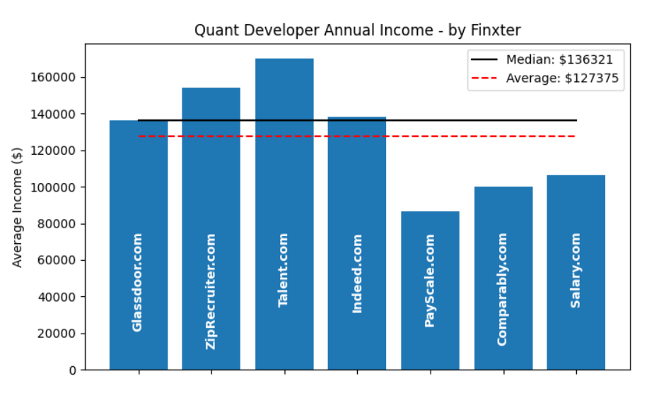
Quantitative developers are some of the best-paid engineers in finance, with compensation varying by location, experience, and employer. In London, junior quant devs often start between £70,000 and £90,000, while mid-level developers earn £120,000 to £180,000. Senior positions at investment banks, hedge funds, or proprietary trading firms frequently exceed £200,000, with contractors sometimes billing £700 to £1,200 per day outside IR35. In New York, salaries are even higher: entry-level roles typically fall in the $100,000 to $130,000 range, mid-level developers earn $150,000 to $200,000, and senior hires at top hedge funds can reach $250,000 to $400,000+.

Total compensation is usually boosted by bonuses, which can be very significant in high-performing funds or trading desks. While banks generally offer slightly lower pay in exchange for stability, hedge funds and prop shops provide the highest upside, and fintechs often compete with equity packages instead of cash. Contractors benefit from flexibility and higher daily rates but give up job security and benefits. Within the field, specialization also plays a role: C++ developers working on low-latency trading systems command the strongest salaries, while Python-focused developers, though still well paid, typically earn a bit less. Across regions, U.S. pay tends to outpace European markets, but in every case, quant developers consistently earn well above typical software engineering salaries, reflecting the critical role their work plays in moving global markets.

4. How is the job market for them?

global financial hubs. Investment banks continue to hire them to build and maintain risk engines and pricing platforms, while hedge funds and proprietary trading firms aggressively expand their low-latency trading teams. At the same time, fintech startups and crypto/DeFi firms are creating new demand for developers who can combine finance, data, and engineering skills.

Demand is strongest in cities like London, New York, Hong Kong, and Chicago, with Zurich, Frankfurt, Singapore, and Tokyo also offering strong markets for risk and trading specialists. Employers are especially eager to find C++ developers skilled in performance and latency optimization, while Python developers remain in high demand for data pipelines, prototyping, and machine learning applications.

Experience with distributed systems, cloud platforms, and real-time data processing makes candidates even more competitive. The rise of machine learning in finance has also created hybrid roles that blend software engineering with data science. Job stability tends to be highest at banks, while the biggest upside is offered by hedge funds and prop shops, which often compete fiercely for top candidates by raising salaries.

Contracting opportunities remain strong in London, with high day rates and flexibility, although these roles come with less security. Overall, the market is robust and demand consistently outpaces supply, making skilled quant developers highly valuable in a world where speed, accuracy, and innovation are central to financial success.

5. Conclusion

In conclusion, the role of the quantitative developer has become indispensable in modern finance.
They sit at the intersection of mathematics, software engineering, and financial markets, transforming theory into production-ready systems.
Their work underpins trading platforms, risk engines, pricing libraries, and portfolio analytics.
Without quant developers, many of the models designed by quantitative analysts would remain purely academic.
The profession combines deep technical expertise with financial intuition, a rare and valuable mix.
It is also one of the few roles where C++ mastery continues to provide a strong competitive edge.
At the same time, Python has cemented its place as the language of choice for rapid prototyping and data analysis.
The career offers exceptional compensation, with salaries and day rates far exceeding traditional software roles.
But beyond money, it provides intellectual challenge and direct market impact.
Each line of code written by a quant dev has the potential to influence millions in PnL or mitigate significant risks.
The job market remains strong, with demand outpacing supply across banks, hedge funds, and fintechs.
Global hubs like London, New York, Hong Kong, and Chicago will continue to attract top talent.
Meanwhile, the rise of machine learning, cloud computing, and decentralized finance is expanding the scope of opportunities.
Quant developers are no longer confined to traditional institutions—they are shaping the future of fintech and digital assets.
Those who excel combine low-level performance engineering with an ability to adapt to new paradigms.
The best quant devs are lifelong learners, constantly updating their skills in algorithms, systems, and finance.
For aspiring professionals, it is a career that rewards curiosity, rigor, and resilience.
For the industry, it is a role that ensures innovation and stability in equal measure.
Ultimately, quantitative developers are the engineers behind modern markets, ensuring that complex ideas can operate at scale.
Their contribution is both foundational and forward-looking, making them central to the evolution of global finance.

August 23, 2025 0 comments

Multithreading in C++ for Quantitative Finance

by cppforquants August 23, 2025

Multithreading in C++ is one of those topics that every developer eventually runs into, whether they’re working in finance, gaming, or scientific computing. The language gives you raw primitives, but it also integrates with a whole ecosystem of libraries that scale from a few threads on your laptop to thousands of cores in a data center.

Choosing the right tool matters: what are the right libraries for your quantitative finance use case?

Multithreading in C++

1. Standard C++ Threads (Low-Level Control)

Since C++11, <thread>, <mutex>, and <future> are part of the standard. You manage threads directly, making it portable and dependency-free.

Example: Parallel computation of moving averages in a trading engine

#include <iostream>
#include <thread>
#include <vector>

void moving_average(const std::vector<double>& data, int start, int end) {
    for (int i = start; i < end; i++) {
        if (i >= 2) {
            double avg = (data[i] + data[i-1] + data[i-2]) / 3.0;
            std::cout << "Index " << i << " avg = " << avg << "\n";
        }
    }
}

int main() {
    std::vector<double> prices = {100,101,102,103,104,105,106,107};
    std::thread t1(moving_average, std::ref(prices), 0, 4);
    std::thread t2(moving_average, std::ref(prices), 4, prices.size());

    t1.join();
    t2.join();
}

2. Intel oneTBB (Task-Based Parallelism)

oneTBB (Threading Building Blocks) provides parallel loops, pipelines, and task graphs. Perfect for HPC or financial risk simulations.

Example: Monte Carlo option pricing

#include <tbb/parallel_for.h>
#include <vector>
#include <random>

int main() {
    const int N = 1'000'000;
    std::vector<double> results(N);

    std::mt19937 gen(42);
    std::normal_distribution<> dist(0, 1);

    tbb::parallel_for(0, N, [&](int i) {
        double z = dist(gen);
        results[i] = std::exp(-0.5 * z * z); // toy payoff
    });
}

3. OpenMP (Loop Parallelism for HPC)

OpenMP is widely used in scientific computing. You add pragmas, and the compiler generates parallel code.

#include <vector>
#include <omp.h>

int main() {
    const int N = 500;
    std::vector<std::vector<double>> A(N, std::vector<double>(N, 1));
    std::vector<std::vector<double>> B(N, std::vector<double>(N, 2));
    std::vector<std::vector<double>> C(N, std::vector<double>(N, 0));

    #pragma omp parallel for
    for (int i = 0; i < N; i++)
        for (int j = 0; j < N; j++)
            for (int k = 0; k < N; k++)
                C[i][j] += A[i][k] * B[k][j];
}

4. Boost.Asio (Async Networking and Thread Pools)

Boost.Asio is ideal for low-latency servers, networking, and I/O-heavy workloads (e.g. trading gateways).

#include <boost/asio.hpp>
using boost::asio::ip::tcp;

int main() {
    boost::asio::io_context io;
    tcp::acceptor acceptor(io, tcp::endpoint(tcp::v4(), 12345));

    std::function<void()> do_accept = [&]() {
        auto socket = std::make_shared<tcp::socket>(io);
        acceptor.async_accept(*socket, [&, socket](boost::system::error_code ec) {
            if (!ec) {
                boost::asio::async_read_until(*socket, boost::asio::dynamic_buffer(std::string()), '\n',
                    [socket](auto, auto) {
                        boost::asio::write(*socket, boost::asio::buffer("pong\n"));
                    });
            }
            do_accept();
        });
    };

    do_accept();
    io.run();
}

5. Parallel STL (`<execution>`)

C++17 added execution policies for standard algorithms. This makes parallelism easy.

#include <algorithm>
#include <execution>
#include <vector>

int main() {
    std::vector<int> trades = {5,1,9,3,2,8};
    std::sort(std::execution::par, trades.begin(), trades.end());
}

6. Conclusion

Multithreading in C++ offers many models, each fit for different workloads. Use std::thread for low-level control of system tasks. Adopt oneTBB or OpenMP for data-parallel HPC simulations. Leverage Boost.Asio for async networking and trading engines. Rely on CUDA/SYCL for GPU acceleration in Monte Carlo or ML. Enable Parallel STL (<execution>) for easy speed-ups in modern code. Try actor frameworks (CAF/HPX) for distributed, message-driven systems.

Compiler flags also make a big difference in multithreaded performance. Always build with -O3 -march=native (or /O2 in MSVC). Use -fopenmp or link to TBB scalable allocators when relevant. Prevent false sharing with alignas(64) and prefer thread_local scratchpads. Mark non-aliasing pointers with __restrict__ to help vectorization. Consider specialized allocators (jemalloc, TBB) in multi-threaded apps. Profile with -fsanitize=thread to catch race conditions early.

The key: match the concurrency model + compiler setup to your workload for maximum speed.

August 23, 2025 0 comments

Risk

What Is DV01? An Implementation in C++

by cppforquants July 26, 2025

What is DV01? In fixed income markets, DV01 (Dollar Value of 01) is one of the most important risk measures every quant, trader, and risk manager needs to understand. DV01 tells you how much the price of a bond, swap, or portfolio changes when interest rates shift by just one basis point (0.01%). This tiny movement in yield can translate into thousands or even millions of dollars in profit or loss for large portfolios.

In other words, DV01 measures interest rate sensitivity in dollar terms. If you’ve ever wondered “What is DV01 in bonds?”, think of it as the financial system’s ruler for measuring how prices react to micro-changes in rates.

For quants, DV01 is the foundation for hedging strategies, scenario analysis, and stress testing. For developers, it’s a key calculation baked into trading systems and risk engines. In this article, we’ll explore what DV01 really is, explain the math behind it, and provide a clean, modern C++ implementation to compute DV01 for single bonds and entire portfolios.

What is DV01?

DV01, short for Dollar Value of 01, measures the dollar change in a bond’s price when its yield changes by one basis point (0.01%). It’s derived directly from the bond’s price–yield relationship: when yields rise, bond prices fall, and DV01 quantifies that sensitivity. Mathematically, DV01 is the negative derivative of price with respect to yield, scaled by 1 basis point:

[math] \Large dv01 = – \frac{dP}{dy} \times 0.0001 [/math]

Where:

P = price of the bond (in dollars).
y = yield to maturity (as a decimal, e.g. 0.05 for 5%).
[math] \frac{dP}{dy} [/math] = the rate of change of the bond price with respect to yield (the slope of the price–yield curve).
0.0001 = one basis point expressed as a decimal (1bp = 0.01% = 0.0001).

Example:
A 5-year bond priced at $102 with a modified duration of 4.5 has:

[math] DV01 = 4.5 \times 102 \times 0.0001 = 0.0459 [/math]

This means that if yields go up by just 1bp, the bond’s price will drop by 4.59 cents.

A C++ Implementation

Here is an implementation of a dv01 calcualtion in C++:

#include <iostream>
#include <vector>
#include <cmath>

// --- Bond structure ---
struct Bond {
    double face;      // Face value (e.g. 100)
    double coupon;    // Annual coupon rate (as decimal, e.g. 0.05 for 5%)
    int maturity;     // Maturity in years
    double yield;     // Yield to maturity (as decimal)
};

// --- Price a plain-vanilla annual coupon bond ---
double priceBond(const Bond& bond) {
    double price = 0.0;
    for (int t = 1; t <= bond.maturity; ++t) {
        price += (bond.face * bond.coupon) / std::pow(1 + bond.yield, t);
    }
    price += bond.face / std::pow(1 + bond.yield, bond.maturity); // Add principal repayment
    return price;
}

// --- DV01 using the bump method ---
double dv01(const Bond& bond) {
    constexpr double bp = 0.0001; // One basis point
    double basePrice = priceBond(bond);

    Bond bumpedBond = bond;
    bumpedBond.yield += bp; // bump yield by 1bp

    double bumpedPrice = priceBond(bumpedBond);

    return basePrice - bumpedPrice; // DV01 in dollars
}

// --- Example usage ---
int main() {
    Bond bond = {100.0, 0.05, 5, 0.04}; // Face=100, 5% coupon, 5-year, 4% yield
    double price = priceBond(bond);
    double dv01Value = dv01(bond);

    std::cout << "Bond Price: $" << price << std::endl;
    std::cout << "DV01: $" << dv01Value << std::endl;

    return 0;
}

This simple struct holds the key attributes of a plain-vanilla fixed-rate bond:

Face: The amount the bond will pay back at maturity.
Coupon: Annual interest rate the bond pays.
Maturity: Number of years until final repayment.
Yield: Market-required return, used for discounting future cashflows.

To calculate the dv01 here we:

Takes the original bond price.
Bumps the yield by one basis point (0.0001).
Re-prices the bond using the bumped yield.
Subtracts the bumped price from the original price.

This gives the DV01 the measures how much the price changes when yields shift by 1bp: this “bump method” is exactly what traders and risk systems use.

Compile and Run

Create dv01.cpp containing the code above, as well as a CMakeLists.txt like:

cmake_minimum_required(VERSION 3.10)
project(dv01)
set(CMAKE_CXX_STANDARD 17)
add_executable(dv01 ../dv01.cpp)

Then run the compilation:

mkdir build
cd build
cmake ..
make

Then run the program:

./dv01
Bond Price: $104.452
DV01: $0.0457561

The code of the application is accessible here:

https://github.com/cppforquants/dv01

Alternative Implementations

When moving from educational examples to real-world analytics, most teams don’t maintain their own pricing code: they turn to professional libraries. In C++, the dominant choice is QuantLib, an open-source framework used by banks, hedge funds, and trading desks worldwide. QuantLib offers several advantages for calculating bond price sensitivity:

It handles all the details you would otherwise code by hand, including calendars, settlement dates, and day count conventions.
It includes a wide range of pricing engines, so the same approach works for fixed-rate bonds, floaters, swaps, and even more complex instruments.
It allows you to shift the yield curve directly and reprice instantly, so bumping rates for sensitivity tests is just a matter of swapping in a different term structure.
It ensures consistency with market standards, which is critical if your numbers need to match the desk’s systems.

For a teaching example, writing the pricing loop yourself is helpful… But for production, using QuantLib means fewer bugs, faster development, and calculations that match what traders and risk managers expect.

#include <ql/quantlib.hpp>
#include <iostream>

using namespace QuantLib;

int main() {
    try {
        // 1. Set the evaluation date
        Calendar calendar = TARGET();
        Date today(26, July, 2025);
        Settings::instance().evaluationDate() = today;

        // 2. Define bond parameters
        Date maturity(26, July, 2030);
        Real faceAmount = 100.0;
        Rate couponRate = 0.05; // 5% annual coupon

        // 3. Build the bond schedule
        Schedule schedule(today, maturity, Period(Annual), calendar,
                          Unadjusted, Unadjusted, DateGeneration::Forward, false);

        // 4. Create the fixed-rate bond
        FixedRateBond bond(3, faceAmount, schedule,
                           std::vector<Rate>{couponRate},
                           ActualActual(ActualActual::ISDA));

        // 5. Build the flat yield curve at 4%
        Handle<YieldTermStructure> curve(
            boost::make_shared<FlatForward>(today, 0.04, ActualActual(ActualActual::ISDA)));

        // 6. Attach a discounting engine
        bond.setPricingEngine(boost::make_shared<DiscountingBondEngine>(curve));

        // 7. Compute base price
        Real basePrice = bond.cleanPrice();

        // 8. Bump the yield curve by 1bp (0.01%) and reprice
        Handle<YieldTermStructure> bumpedCurve(
            boost::make_shared<FlatForward>(today, 0.0401, ActualActual(ActualActual::ISDA)));
        bond.setPricingEngine(boost::make_shared<DiscountingBondEngine>(bumpedCurve));

        Real bumpedPrice = bond.cleanPrice();

        // 9. Compute and print sensitivity
        Real priceChange = basePrice - bumpedPrice;

        std::cout << "Base Price: " << basePrice << std::endl;
        std::cout << "Price Change for 1bp shift: " << priceChange << std::endl;
    }
    catch (std::exception& e) {
        std::cerr << "Error: " << e.what() << std::endl;
        return 1;
    }

    return 0;
}

To run the example, install QuantLib (for example, via your system package manager or by building from source) and compile with a standard C++17 or later compiler:

g++ -std=c++17 -I/usr/include/ql -lQuantLib sensitivity_example.cpp -o sensitivity_example
./sensitivity_example

This produces the base bond price and the change in price after a 1bp shift in the yield curve. From there, you can expand the approach:

Price a portfolio of bonds by looping through multiple instruments and summing their sensitivities.
Swap in a different term structure (e.g., a real yield curve from market data) to see how results change under new scenarios.
Experiment with different bond types like floaters or callable bonds by just changing the instrument class and pricing engine.

These extensions show how the same core idea can scale from a single-bond demo into a risk engine component that handles thousands of securities and multiple yield environments.

July 26, 2025 0 comments

Greeks

How to Calculate Theta for Options in C++

by cppforquants July 19, 2025

In quantitative finance, understanding how an option’s value changes over time is critical for risk management and trading. This is where Theta, the Greek that measures time decay, plays a central role. In this article, you’ll learn how to calculate Theta for options in C++ with a simple yet powerful approach to estimate how much an option’s price erodes as it approaches expiration. Whether you’re building a pricing engine or just deepening your understanding of the Greeks, this guide will walk you through a practical C++ implementation step-by-step.

Theta for Options Explained

1. What is Theta?

Theta is one of the most important Greeks in options trading. It measures the rate at which an option loses value as time passes, assuming all other factors remain constant. This phenomenon is known as time decay.

Mathematically, Theta is defined as the partial derivative of the option price V with respect to time t:

[math]\large \Theta = \frac{\partial V}{\partial t}[/math]

In most practical cases, Theta is negative for long option positions meaning the value of the option decreases as time progresses. This reflects the diminishing probability that the option will end up in-the-money as expiration nears.

Imagine you hold a European call option on a stock priced at $100, with a strike at $100 and 30 days to expiry. If the option is worth $4.00 today, and $3.95 tomorrow (with no change in volatility or the stock price), then Theta is approximately:

[math]\large \Theta \approx \frac{3.95 – 4.00}{1} = -0.05[/math]

This means the option loses 5 cents per day due to the passage of time alone.

Key Characteristics of Theta:

Short-term options have higher Theta (faster decay).
At-the-money options typically experience the highest Theta.
Theta increases as expiration approaches, especially in the final weeks.
Call and put options both exhibit Theta decay, but not symmetrically.

2. The Black-Scholes Formula

Under the Black-Scholes model, we can calculate Theta analytically for both European call and put options. These closed-form expressions are widely used for pricing, calibration, and risk reporting.

Black-Scholes Theta Formulas

European Call Option Theta:

[math]\large \Theta_{\text{call}} = -\frac{S \cdot \sigma \cdot N'(d_1)}{2\sqrt{T}} – rK e^{-rT} N(d_2)[/math]

European Put Option Theta:

[math]\large \Theta_{\text{put}} = -\frac{S \cdot \sigma \cdot N'(d_1)}{2\sqrt{T}} + rK e^{-rT} N(-d_2)[/math]

Where:

[math]S[/math] = spot price of the underlying
[math]K[/math] = strike price
[math]T[/math] = time to maturity (in years)
[math]r[/math] = risk-free interest rate
[math]\sigma[/math] = volatility
[math]N(d)[/math] = cumulative normal distribution
[math]N'(d)[/math] = standard normal density (i.e., PDF)
[math]d_1 = \frac{\ln(S/K) + (r + \sigma^2/2)T}{\sigma \sqrt{T}}[/math]

3. An Implementation in C++

Here’s a minimal, self-contained example that calculates Theta using QuantLib:

#include <ql/quantlib.hpp>
#include <iostream>

using namespace QuantLib;

int main() {
    // Set evaluation date
    Calendar calendar = TARGET();
    Date today(19, July, 2025);
    Settings::instance().evaluationDate() = today;

    // Option parameters
    Option::Type optionType = Option::Call;
    Real underlying = 100.0;
    Real strike = 100.0;
    Rate riskFreeRate = 0.01;     // 1%
    Volatility volatility = 0.20; // 20%
    Date maturity = calendar.advance(today, 90, Days); // 3 months
    DayCounter dayCounter = Actual365Fixed();

    // Construct option
    ext::shared_ptr<Exercise> europeanExercise(new EuropeanExercise(maturity));
    ext::shared_ptr<StrikedTypePayoff> payoff(new PlainVanillaPayoff(optionType, strike));
    VanillaOption europeanOption(payoff, europeanExercise);

    // Market data (handle wrappers)
    Handle<Quote> spot(ext::shared_ptr<Quote>(new SimpleQuote(underlying)));
    Handle<YieldTermStructure> flatRate(ext::shared_ptr<YieldTermStructure>(
        new FlatForward(today, riskFreeRate, dayCounter)));
    Handle<BlackVolTermStructure> flatVol(ext::shared_ptr<BlackVolTermStructure>(
        new BlackConstantVol(today, calendar, volatility, dayCounter)));

    // Black-Scholes-Merton process
    ext::shared_ptr<BlackScholesMertonProcess> bsmProcess(
        new BlackScholesMertonProcess(spot, flatRate, flatRate, flatVol));

    // Set pricing engine
    europeanOption.setPricingEngine(ext::shared_ptr<PricingEngine>(
        new AnalyticEuropeanEngine(bsmProcess)));

    // Output results
    std::cout << "Option price: " << europeanOption.NPV() << std::endl;
    std::cout << "Theta (per year): " << europeanOption.theta() << std::endl;
    std::cout << "Theta (per day): " << europeanOption.theta() / 365.0 << std::endl;

    return 0;
}

This example prices a European call option using QuantLib’s AnalyticEuropeanEngine, which leverages the Black-Scholes formula to compute both the option’s price and its Greeks, including Theta. The method theta() returns the annualized Theta value, representing the rate of time decay per year; dividing it by 365 gives the daily Theta, which is more intuitive for short-term trading and hedging. You can easily experiment with other scenarios by changing the option type to Option::Put or adjusting the maturity date to observe how Theta behaves under different conditions.

4. Compile and Run

You will need to install Quantlib first, on a mac:

brew install quantlib

and then prepare your CMakeList.txt:

cmake_minimum_required(VERSION 3.10)
project(theta)

set(CMAKE_CXX_STANDARD 17)

find_package(PkgConfig REQUIRED)
pkg_check_modules(QUANTLIB REQUIRED QuantLib)

include_directories(${QUANTLIB_INCLUDE_DIRS})
link_directories(${QUANTLIB_LIBRARY_DIRS})

add_executable(theta ../theta.cpp)
target_link_libraries(theta ${QUANTLIB_LIBRARIES})

Where theta.cpp contains the code from the former section.

Then:

mkdir build
cd build
cmake..
make

Once compiled, you can run the executable:

➜  build git:(main) ✗ ./theta
Option price: 4.65065
Theta (per year): -6.73569

Which gives you the value of theta.

You can clone the project here on Github to calculate Theta for options in C++:

https://github.com/cppforquants/theta

July 19, 2025 0 comments

Interview

Non-Overlapping Intervals in C++: A Quantitative Developer Interview Question

by cppforquants July 13, 2025

In quantitative developer interviews, you’re often tested not just on algorithms, but on how they apply to real-world financial systems. One common scenario: cleaning overlapping time intervals from noisy market data feeds. This challenge maps directly to LeetCode 435: Non-Overlapping Intervals. In this article, we’ll solve it in C++ and explore why it matters in quant finance from ensuring data integrity to preparing time series for model training. How to solve the problem of non-overlapping intervals in C++?

Let’s dive into a practical problem that tests both coding skill and quant context.

1. Problem Statement

You’re given a list of intervals, where each interval represents a time range during which a market data feed was active. Some intervals may overlap, resulting in duplicated or conflicting data.

Your task is to determine the minimum number of intervals to remove so that the remaining intervals do not overlap. The goal is to produce a clean, non-overlapping timeline: a common requirement in financial data preprocessing.

Input: intervals = {{1,3}, {2,4}, {3,5}, {6,8}}
Output: 1

Explanation: Removing {2,4} results in non-overlapping intervals: {{1,3}, {3,5}, {6,8}}.

2. The Solution Explained

To remove the fewest intervals and eliminate overlaps, we take a greedy approach: we always keep the interval that ends earliest, since this leaves the most room for future intervals.

By sorting all intervals by their end time, we can iterate through them and:

Keep an interval if it doesn’t overlap with the last selected one.
Remove it otherwise.

This strategy ensures we keep as many non-overlapping intervals as possible and thus remove the minimum necessary.

What is the time and space complexity for this approach?

Sorting dominates the time complexity. While the actual iteration through the intervals is linear (O(n)), sorting the n intervals takes O(nlogn), and that becomes the bottleneck.

Although we process all n intervals, we do so in place without allocating any extra data structures. We use just a few variables (last_end, removed), so the auxiliary space remains constant. That’s why the space complexity is O(1) assuming the input list is already given and we’re allowed to sort it directly.

Aspect	Value	Explanation

Time Complexity

O(n log n)

Due to sorting the intervals by end time

Space Complexity

O(1) (excluding input)

Only a few variables used; no extra data structures needed

Now, let’s implement it in C++.

3. A C++ Implementation

Here is a C++ implementation of the solution:

#include <iostream>
#include <vector>
#include <algorithm>
#include <climits>
using namespace std;

// Greedy function to compute the minimum number of overlapping intervals to remove
int eraseOverlapIntervals(vector<vector<int>>& intervals) {
    // Sort intervals by end time
    sort(intervals.begin(), intervals.end(), [](const auto& a, const auto& b) {
        return a[1] < b[1];
    });

    int removed = 0;
    int last_end = INT_MIN;

    for (const auto& interval : intervals) {
        if (interval[0] < last_end) {
            // Overlapping — must remov.e this one
            removed++;
        } else {
            // No overlap — update last_end
            last_end = interval[1];
        }
    }

    return removed;
}

int main() {
    vector<vector<int>> intervals = {{1, 3}, {2, 4}, {3, 5}, {6, 8}};
    int result = eraseOverlapIntervals(intervals);
    cout << "Minimum intervals to remove: " << result << endl;
    return 0;
}

Let’s compile:

mkdir build
cmake ..
make

And run the code:

➜  build git:(main) ✗ ./intervals
Minimum intervals to remove: 1

4. Do It Yourself

To do it yourself, you can clone my repository to solve non-overlapping intervals in C++here:

https://github.com/cppforquants/overlappingintervals

Just git clone and run the compilation/execution commands from the Readme:

# Overlapping Intervals

The overlapping intervals problem for quant interviews.

## Build

```bash
mkdir build
cd build
cmake ..
make
```

## Run
```
./intervals

July 13, 2025 0 comments

Performance

Memory Management in C++ High-Frequency Trading Systems

by cppforquants July 12, 2025

High-Frequency Trading (HFT) systems operate under extreme latency constraints where microseconds matter. In this environment, memory management is not just an implementation detail. The ability to predict and control memory allocations, avoid page faults, minimize cache misses, and reduce heap fragmentation can directly influence trading success. What are the best tricks for memory management in C++?

C++ offers low-level memory control unmatched by most modern languages, making it a staple in the HFT tech stack. However, this power comes with responsibility: careless allocations or unexpected copies can introduce jitter, latency spikes, and subtle bugs that are unacceptable in production systems.

In this article, we’ll explore how memory management principles apply in HFT, the common patterns and pitfalls, and how to use modern C++ tools to build robust, deterministic, and lightning-fast trading systems.

1. Preallocation and Memory Pools

A common mitigation strategy is preallocating memory up front and using a memory pool to manage object lifecycles efficiently. This approach ensures allocations are fast, deterministic, and localized, which also improves cache performance.

Let’s walk through a simple example using a custom fixed-size memory pool.

C++ Example: Fixed-Size Memory Pool for Order Objects

#include <iostream>
#include <vector>
#include <bitset>
#include <cassert>

constexpr size_t MAX_ORDERS = 1024;

struct Order {
    int id;
    double price;
    int quantity;

    void reset() {
        id = 0;
        price = 0.0;
        quantity = 0;
    }
};

class OrderPool {
public:
    OrderPool() {
        for (size_t i = 0; i < MAX_ORDERS; ++i) {
            free_slots.set(i);
        }
    }

    Order* allocate() {
        for (size_t i = 0; i < MAX_ORDERS; ++i) {
            if (free_slots.test(i)) {
                free_slots.reset(i);
                return &orders[i];
            }
        }
        return nullptr; // Pool exhausted
    }

    void deallocate(Order* ptr) {
        size_t index = ptr - orders;
        assert(index < MAX_ORDERS);
        ptr->reset();
        free_slots.set(index);
    }

private:
    Order orders[MAX_ORDERS];
    std::bitset<MAX_ORDERS> free_slots;
};

Performance Benefits:

No heap allocation: All Order objects are stack-allocated as part of the orders array.
O(1) deallocation: Releasing an object is just a bitset flip and a reset.
Cache locality: Contiguous storage means fewer cache misses during iteration.

2. Object Reuse and Freelist Patterns

Even with preallocated memory, repeatedly constructing and destructing objects introduces CPU overhead and memory churn. In HFT systems, where throughput is immense and latency must be consistent, reusing objects via a freelist is a proven strategy to reduce jitter and improve performance via a simple trick of memory management in C++.

A freelist is a lightweight structure that tracks unused objects for quick reuse. Instead of releasing memory, objects are reset and pushed back into the freelist for future allocations: a near-zero-cost operation.

C++ Example: Freelist for Reusing Order Objects

#include <iostream>
#include <stack>

struct Order {
    int id;
    double price;
    int quantity;

    void reset() {
        id = 0;
        price = 0.0;
        quantity = 0;
    }
};

class OrderFreelist {
public:
    Order* acquire() {
        if (!free.empty()) {
            Order* obj = free.top();
            free.pop();
            return obj;
        }
        return new Order();  // Fallback allocation
    }

    void release(Order* obj) {
        obj->reset();
        free.push(obj);
    }

    ~OrderFreelist() {
        while (!free.empty()) {
            delete free.top();
            free.pop();
        }
    }

private:
    std::stack<Order*> free;
};

Performance Benefits:

Reusing instead of reallocating: Objects are reset, not destroyed — drastically reduces allocation pressure.
Stack-based freelist: LIFO behavior benefits CPU cache reuse due to temporal locality (recently used objects are reused soon).
Amortized heap usage: The heap is only touched when the freelist is empty, which should rarely happen in a tuned system.

3. Use Arena Allocators

When stack allocation isn’t viable — e.g., for large datasets or objects with dynamic lifetimes — heap usage becomes necessary. But in HFT, direct new/delete or malloc/free calls are risky due to latency unpredictability and fragmentation.

This is where placement new and arena allocators come into play.

Placement new gives you explicit control over where an object is constructed.
Arena allocators preallocate a large memory buffer and dole out chunks linearly, eliminating the overhead of general-purpose allocators and enabling bulk deallocation.

These techniques are foundational for building fast, deterministic allocators in performance-critical systems like trading engines and improve memory management in C++.

C++ Example: Arena Allocator with Placement new

#include <iostream>
#include <vector>
#include <cstdint>
#include <new>      // For placement new
#include <cassert>

constexpr size_t ARENA_SIZE = 4096;

class Arena {
public:
    Arena() : offset(0) {}

    void* allocate(size_t size, size_t alignment = alignof(std::max_align_t)) {
        size_t aligned_offset = (offset + alignment - 1) & ~(alignment - 1);
        if (aligned_offset + size > ARENA_SIZE) {
            return nullptr; // Out of memory
        }
        void* ptr = &buffer[aligned_offset];
        offset = aligned_offset + size;
        return ptr;
    }

    void reset() {
        offset = 0; // Bulk deallocation
    }

private:
    alignas(std::max_align_t) char buffer[ARENA_SIZE];
    size_t offset;
};

// Sample object to construct inside arena
struct Order {
    int id;
    double price;
    int qty;

    Order(int i, double p, int q) : id(i), price(p), qty(q) {}
};

Performance Benefits

Deterministic allocation: Constant-time, alignment-safe, no system heap calls.
Zero-cost deallocation: arena.reset() clears all allocations in one go — no destructor calls, no fragmentation.
Minimal overhead: Perfect for short-lived objects in bursty, time-sensitive workloads.

Ideal Use Cases in HFT

Message parsing and object hydration (e.g., FIX messages → Order objects).
Per-frame or per-tick memory lifetimes.
Temporary storage in pricing or risk models where objects live for microseconds.

4. Use Custom Allocators in STL (e.g., `std::pmr`)

Modern C++ introduced a powerful abstraction for memory control in the standard library: polymorphic memory resources (std::pmr). This allows you to inject custom memory allocation behavior into standard containers like std::vector, std::unordered_map, etc., without writing a full custom allocator class.

This is especially valuable in HFT where STL containers may be needed temporarily (e.g., per tick or per packet) and where you want tight control over allocation patterns, lifetime, and performance.

C++ Example: Using std::pmr::vector with an Arena

#include <iostream>
#include <memory_resource>
#include <vector>
#include <string>

int main() {
    constexpr size_t BUFFER_SIZE = 1024;
    char buffer[BUFFER_SIZE];

    // Set up a monotonic buffer resource using stack memory
    std::pmr::monotonic_buffer_resource resource(buffer, BUFFER_SIZE);

    // Create a pmr vector that uses the custom memory resource
    std::pmr::vector<std::string> symbols{&resource};

    // Populate the vector
    symbols.emplace_back("AAPL");
    symbols.emplace_back("MSFT");
    symbols.emplace_back("GOOG");

    for (const auto& s : symbols) {
        std::cout << s << "\n";
    }

    // All memory is deallocated at once when `resource` goes out of scope or is reset
}

Benefits for HFT Systems

Scoped allocations: The monotonic_buffer_resource allocates from the buffer and never deallocates until reset — perfect for short-lived containers (e.g., market snapshots).
No heap usage: Memory is pulled from the stack or a preallocated slab, avoiding malloc/free.
STL compatibility: Works with all std::pmr:: containers (vector, unordered_map, string, etc.).
Ease of integration: Drop-in replacement for standard containers — no need to write full allocator classes.

pmr Design Philosophy

Polymorphic behavior: Containers store a pointer to an std::pmr::memory_resource, enabling allocator reuse without changing container types.
Composable: You can plug in arenas, pools, fixed-size allocators, or even malloc-based resources depending on the use case.

Common pmr Resources

Resource	Use Case
`monotonic_buffer_resource`	Fast, one-shot allocations (e.g., per tick)
`unsynchronized_pool_resource`	Small object reuse with subpooling (no mutex)
`synchronized_pool_resource`	Thread-safe version of above
Custom	Arena/slab allocators for domain-specific control

July 12, 2025 0 comments

Jobs

Best Hedge Funds For Quantitative Developers

by cppforquants July 10, 2025

In 2025, a select cohort of hedge funds and prop trading firms is fiercely competing for elite quantitative developers—those adept in coding, statistics, and machine learning. Firms like Citadel, D.E. Shaw, Two Sigma, and others are leading the charge, offering six‑figure base salaries and performance bonuses tied directly to alpha generated. What are the best hedge funds for quantitative developers?

1. Citadel

Citadel and Citadel Securities continue their aggressive recruitment, launching intensive internship pipelines with record-low acceptance rates (0.4%) to secure the next generation of quant talent. Summer interns can earn as much as $5,000 per week—an early indicator of the hyper-competitive environment. With approximately $65 billion in assets under management, the firm is deeply reliant on advanced technology, and quant developers play a central role in driving trading decisions, building low-latency systems, and maintaining scalable infrastructure. Citadel’s recruitment is global, with open roles in major financial hubs like New York, London, Miami, Gurugram, and Hong Kong.

Citadel’s hiring funnel is notoriously selective. Their internship program, a key gateway to full-time roles, had a 0.4% acceptance rate this year—more competitive than top-tier tech firms. Interns can earn up to $24,000 per month, reflecting the high value Citadel places on early talent. These internships are intensive and structured to transition into permanent positions quickly.

Full-time quantitative developer roles offer some of the highest compensation in the industry, with total packages ranging from $200,000 to over $700,000 per year, and a median near $550,000. Citadel Securities, the firm’s market-making division, offers similarly lucrative packages for developer positions focused on execution engines and infrastructure.

The firm places a premium on engineers with strong coding ability in C++, Python, and systems-level programming, as well as deep understanding of algorithms, data structures, and statistics. Citadel is expanding in regions like India, particularly targeting IIT graduates for roles in equity derivatives technology.

2. D.E. Shaw

D.E. Shaw remains one of the most prestigious and desirable hedge funds hiring quantitative developers. Founded in 1988, the firm has built its reputation on rigorous research, engineering excellence, and a collaborative, low-ego culture that appeals strongly to top STEM graduates and seasoned engineers alike. With offices in New York, London, and Hyderabad, D.E. Shaw offers global opportunities for quant devs to work on high-impact systems supporting both systematic and discretionary trading strategies.

Quantitative developers at D.E. Shaw are deeply embedded in cross-functional teams, partnering closely with researchers and portfolio managers. They build and optimize everything from execution platforms and backtesting frameworks to pricing engines and large-scale data ingestion systems. The firm’s approach is highly academic, often drawing in PhDs in computer science, physics, and mathematics, but equally welcoming experienced software engineers from top tech firms.

The firm’s hiring process is known for being intellectually demanding but fair, focusing on algorithmic problem solving, systems design, and real-world coding skills. Compensation is highly competitive, with total packages for junior developers often exceeding $400,000 and rising quickly with experience. Unlike some more aggressive competitors, D.E. Shaw places a greater emphasis on long-term innovation and internal mobility, rather than rapid iteration.

D.E. Shaw continues to prioritize talent development through structured mentorship, technical training, and a strong internal engineering culture. The firm is particularly attractive to candidates who value technical depth, thoughtful problem solving, and a strong sense of intellectual camaraderie. In 2025, it remains a top-tier choice for quant developers seeking a high-impact, research-driven engineering career in finance.

3. Two Sigma

In 2025, Two Sigma continues to distinguish itself as one of the most engineering-driven hedge funds hiring quantitative developers. Based in New York with a global presence, the firm operates at the intersection of finance, data science, and cutting-edge software engineering. Unlike some peers that prioritize trading speed above all, Two Sigma is renowned for its research-first culture and thoughtful approach to building scalable, maintainable systems that support a wide range of data-driven investment strategies.

Quant developers at Two Sigma are more than infrastructure engineers—they build the platforms, tools, and pipelines that power research and trading. From developing custom machine learning frameworks to managing terabytes of alternative data, their work enables researchers to test hypotheses at scale and deploy production strategies with minimal friction. This blend of software craftsmanship and statistical rigor makes Two Sigma a magnet for developers from Google, Meta, and top academic institutions.

The hiring process is structured around deep technical assessments, covering data structures, algorithms, distributed systems, and applied ML. Interviews are known for being intense but well-organized, with an emphasis on real-world engineering challenges rather than trick questions. Compensation is highly attractive, with total packages for mid-level developers typically ranging from $400K to $600K, along with generous perks and equity-like incentives.

Two Sigma’s engineering culture is known for its clean code, peer reviews, mentorship, and internal tooling excellence. It is particularly appealing to developers who want to work in a rigorous yet collaborative environment where the long-term quality of systems matters as much as short-term gains. For quantitative developers who value a balance of intellectual depth, modern software practices, and strong research collaboration, Two Sigma remains one of the most desirable destinations in 2025.

4. Jump Trading

Jump Trading ranks among the top hedge funds aggressively hiring quantitative developers, particularly those with expertise in low-latency systems and high-performance computing. Headquartered in Chicago with key offices in London, Singapore, and New York, Jump operates as a technology-centric trading firm where developers play a foundational role in shaping the firm’s competitive edge in high-frequency markets.

Quantitative developers at Jump are responsible for building ultra-low-latency trading infrastructure, co-located exchange connectivity, and high-throughput data pipelines. The work is performance-critical—developers routinely optimize nanosecond-level latency in C++, tune networking stacks, and architect systems that process millions of messages per second. This makes Jump a prime destination for engineers who thrive on precision, speed, and scale.

Jump’s hiring process is notoriously rigorous. The firm recruits from the most elite technical talent pools—top-tier CS programs, Olympiad medalists, and systems engineers from Google, Meta, and Nvidia. Interviews emphasize C++ mastery, concurrency, networking, and real-time system design. Candidates should expect deep-dive technical sessions with a strong focus on engineering fundamentals and execution under pressure.

Compensation at Jump is among the highest in the industry. Total packages for experienced quant devs can reach $700K to $1M+, with highly lucrative performance-based bonuses. Even junior roles offer salaries that rival or exceed those at top tech companies. The firm’s flat structure means that developers can see their work deployed quickly and directly affect P&L.

What sets Jump apart culturally is its research-driven, R&D-focused environment. The firm funds open-source work, sponsors academic research, and even explores crypto markets and digital asset infrastructure through its affiliate, Jump Crypto. For quantitative developers who want to work on bleeding-edge systems in a highly autonomous, deeply technical environment, Jump Trading offers one of the most exciting opportunities in 2025.

5. Hudson River Trading

Hudson River Trading (HRT) stands out as one of the most sought-after firms for quantitative developers seeking a balance between technical excellence, compensation, and culture. Headquartered in New York, HRT is a major player in high-frequency trading, operating across equities, futures, options, and crypto markets. The firm is widely respected for its engineering-first mindset and flat organizational structure, where developers work shoulder-to-shoulder with researchers to build and optimize trading systems from scratch.

Quantitative developers at HRT contribute directly to all layers of the trading stack, including strategy simulation platforms, real-time risk engines, and execution frameworks. The environment demands both creativity and precision—developers frequently write latency-critical C++, build robust Python backtests, and design resilient systems capable of reacting to live market conditions within microseconds. HRT’s infrastructure is primarily built in-house, giving engineers full ownership and the ability to innovate quickly.

The hiring process is designed to identify world-class problem solvers and systems thinkers. Candidates are tested on advanced algorithms, computational efficiency, concurrency, and low-level debugging. HRT regularly recruits from elite programming competitions like the ICPC and Codeforces, and from top computer science programs globally. The interview process is technical and fast-paced, but also fair and transparent.

Compensation is highly competitive. Total compensation for quantitative developers commonly ranges from $350K to $700K+, including generous year-end bonuses tied to firm performance. Despite the fast-moving markets it operates in, HRT is known for maintaining a healthier work-life balance than many of its peers, avoiding the “burnout” culture associated with some HFT firms.

What truly sets HRT apart is its emphasis on high-quality, elegant code and long-term technical investment. The firm fosters a strong sense of developer autonomy and deeply values mentorship, documentation, and code reviews. For quant developers who want to work on mission-critical systems in an environment that values intellect over hierarchy, Hudson River Trading remains a top-tier choice in 2025.

July 10, 2025 0 comments

Libraries

Best C++ Libraries for Matrix Computations

by cppforquants July 5, 2025

Matrix computations are at the heart of many quantitative finance models, from Monte Carlo simulations to risk matrix evaluations. In C++, selecting the right library can dramatically affect performance, readability, and numerical stability. Fortunately, there are several powerful options designed for high-speed computation and scientific accuracy. Whether you need dense, sparse, or banded matrix support, the C++ ecosystem has you covered. Some libraries prioritize speed, others emphasize syntax clarity or Python compatibility. What are the best C++ libraries for matrix computations?

Choosing between Eigen, Armadillo, or Blaze depends on your project goals. If you’re building a derivatives engine or a backtesting framework, using the wrong matrix abstraction can slow you down. In this article, we’ll compare the top C++ matrix libraries, focusing on performance, ease of use, and finance-specific suitability. By the end, you’ll know exactly which one to use for your next quant project. Let’s dive into the best C++ libraries for matrix computations.

1. Eigen

Website: eigen.tuxfamily.org
License: MPL2
Key Features:

Header-only: No linking required
Fast: Competes with BLAS performance
Clean API: Ideal for prototyping and production
Supports: Dense, sparse, and fixed-size matrices
Thread-safe: As long as each thread uses its own objects

Use Case: General-purpose, widely used in finance for risk models and curve fitting.

Eigen is a header-only C++ template library for linear algebra, supporting vectors, matrices, and related algorithms. Known for its performance through expression templates, it’s widely used in quant finance, computer vision, and machine learning.

Here is a snippet example:

#include <iostream>
#include <Eigen/Dense>

int main() {
    // Define 2x2 matrices
    Eigen::Matrix2d A;
    Eigen::Matrix2d B;

    // Initialize matrices
    A << 1, 2,
         3, 4;
    B << 2, 0,
         1, 2;

    // Matrix addition
    Eigen::Matrix2d C = A + B;

    // Matrix multiplication
    Eigen::Matrix2d D = A * B;

    // Print results
    std::cout << "Matrix A + B:\n" << C << "\n\n";
    std::cout << "Matrix A * B:\n" << D << "\n";

    return 0;
}

This is probably one of the best C++ libraries for matrix computations.

2. Armadillo

Website: arma.sourceforge.net
License: MPL2
Key Features:

Readable syntax: Ideal for research and prototyping
Performance-boosted: Uses LAPACK/BLAS when available
Supports: Dense, sparse, banded matrices
Integrates with: OpenMP, ARPACK, SuperLU
Actively maintained: Trusted in academia and finance

Use Case: Quant researchers prototyping algorithms with familiar syntax.

Armadillo is a high-level C++ linear algebra library that offers Matlab-like syntax, making it exceptionally easy to read and write. Under the hood, it can link to BLAS and LAPACK for high-performance computations, especially when paired with libraries like Intel MKL or OpenBLAS.

Here’s a quant finance-style example using Armadillo to perform a Cholesky decomposition on a covariance matrix, which is a common operation in portfolio risk modeling, Monte Carlo simulations, and factor models.

#include <iostream>
#include <armadillo>

int main() {
    using namespace arma;

    // Simulated 3-asset covariance matrix (symmetric and positive-definite)
    mat cov = {
        {0.10, 0.02, 0.04},
        {0.02, 0.08, 0.01},
        {0.04, 0.01, 0.09}
    };

    // Perform Cholesky decomposition: cov = L * L.t()
    mat L;
    bool success = chol(L, cov, "lower");

    if (success) {
        std::cout << "Cholesky factor L:\n";
        L.print();
        
        // Simulate a standard normal vector for 3 assets
        vec z = randn<vec>(3);

        // Generate correlated returns: r = L * z
        vec returns = L * z;

        std::cout << "\nSimulated correlated return vector:\n";
        returns.print();
    } else {
        std::cerr << "Covariance matrix is not positive-definite.\n";
    }

    return 0;
}

3. Blaze

Website: blaze.mathjs.org
License: BSD
Key Features:

Highly optimized: Expression templates + SIMD
Parallel execution: Supports OpenMP, HPX, and pthreads
BLAS backend optional
Supports: Dense/sparse matrices, vectors, custom allocators
Flexible integration: Can plug into existing quant platforms

Use Case: Performance-critical applications like Monte Carlo engines.

Blaze is a high-performance C++ math library that emphasizes speed and scalability. It uses expression templates like Eigen but leans further into parallelism, making it ideal for latency-sensitive finance applications such as pricing engines, curve fitting, or Monte Carlo simulations.

Imagine you simulate 1,000 paths for a European call option across 3 assets. Here’s how you could compute portfolio payoffs using Blaze:

#include <iostream>
#include <blaze/Math.h>

int main() {
    using namespace blaze;

    constexpr size_t numPaths = 1000;
    constexpr size_t numAssets = 3;

    // Simulated terminal prices (rows = paths, cols = assets)
    DynamicMatrix<double> terminalPrices(numPaths, numAssets);
    randomize(terminalPrices);  // Random values between 0 and 1

    // Portfolio weights (e.g., long 1.0 in asset 0, short 0.5 in asset 1, flat in asset 2)
    StaticVector<double, numAssets> weights{1.0, -0.5, 0.0};

    // Compute payoffs: each row dot weights
    DynamicVector<double> payoffs = terminalPrices * weights;

    std::cout << "First 5 simulated portfolio payoffs:\n";
    for (size_t i = 0; i < 5; ++i)
        std::cout << payoffs[i] << "\n";

    return 0;
}

4. xtensor

Website: xtensor.readthedocs.io
License: BSD
Key Features:

Numpy-like multidimensional arrays
Integrates well with Python via xtensor-python
Supports broadcasting and lazy evaluation

Use Case: Interfacing with Python or for higher-dimensional data structures.

xtensor is a C++ library for numerical computing, offering multi-dimensional arrays with NumPy-style syntax. It supports broadcasting, lazy evaluation, and is especially handy for developers needing interoperability with Python (via xtensor-python) or high-dimensional operations in quant research.

Python interop through xtensor-python
Header-only, modern C++17+
Syntax close to NumPy
Fast and memory-efficient
Broadcasting, slicing, views supported

Here is an example for moving average calculation:

#include <iostream>
#include <xtensor/xarray.hpp>
#include <xtensor/xview.hpp>
#include <xtensor/xadapt.hpp>
#include <xtensor/xio.hpp>

int main() {
    using namespace xt;

    // Simulated closing prices (1D tensor)
    xarray<double> prices = {100.0, 101.5, 103.2, 102.0, 104.1, 106.3, 107.5};

    // Window size for moving average
    std::size_t window = 3;

    // Compute moving averages
    std::vector<double> ma_values;
    for (std::size_t i = 0; i <= prices.size() - window; ++i) {
        auto window_view = view(prices, range(i, i + window));
        double avg = mean(window_view)();
        ma_values.push_back(avg);
    }

    // Print result
    std::cout << "Rolling 3-period moving averages:\n";
    for (auto val : ma_values)
        std::cout << val << "\n";

    return 0;
}

Ready for the last entries for our article on the best C++ libraries for matrix computations?

5. FLENS (Flexible Library for Efficient Numerical Solutions)

Website: github.com/michael-lehn/FLENS
License: BSD
Key Features:

Thin wrapper over BLAS/LAPACK for speed
Supports banded and triangular matrices
Good for structured systems in quant PDEs
Integrates well with Fortran-style scientific computing

Use Case: Structured financial models involving PDE solvers.

FLENS is a C++ wrapper around BLAS and LAPACK designed for clear object-oriented syntax and high numerical performance. It provides clean abstractions over dense, sparse, and banded matrices, making it a good fit for quant applications involving curve fitting, linear systems, or differential equations.Object-oriented, math-friendly syntax

Let’s solve a system representing a regression problem (e.g., estimating betas in a factor model):

#include <flens/flens.cxx>
#include <iostream>

using namespace flens;

int main() {
    typedef GeMatrix<FullStorage<double> >   Matrix;
    typedef DenseVector<Array<double> >      Vector;

    // Create matrix A (3x3) and vector b
    Matrix A(3, 3);
    Vector b(3);

    A = 1.0,  0.5,  0.2,
        0.5,  2.0,  0.3,
        0.2,  0.3,  1.0;

    b = 1.0, 2.0, 3.0;

    // Solve Ax = b using LAPACK
    Vector x(b); // solution vector
    lapack::gesv(A, x);  // modifies A and x

    std::cout << "Solution x:\n" << x << "\n";

    return 0;
}

July 5, 2025 0 comments

Volatility

Volatility Smile in C++: An Implementation for Call Options

by cppforquants July 4, 2025

Implied volatility isn’t flat across strikes: it curves. It’s like a smile: the volatility smile.

When plotted against strike price, implied volatilities for call options typically form a smile, with lower volatilities near-the-money and higher volatilities deep in- or out-of-the-money. This shape reflects real-world market dynamics, like the increased demand for tail-risk protection and limitations of the Black-Scholes model.

In this article, we’ll implement a simple C++ tool to compute this volatility smile from observed market prices, helping us visualize and understand its structure.

1. What’s a Volatility Smile?

A volatility smile is a pattern observed in options markets where implied volatility (IV) is not constant across different strike prices — contrary to what the Black-Scholes model assumes. When plotted (strike on the x-axis, IV on the y-axis), the graph forms a smile-shaped curve.

At-the-money (ATM) options tend to have the lowest implied volatility.
In-the-money (ITM) and out-of-the-money (OTM) options show higher implied volatility.

If you plot IV vs. strike price, the shape curves upward at both ends, resembling a smile.

Implied volatility is lowest near the at-the-money (ATM) strike and increases for both in-the-money (ITM) and out-of-the-money (OTM) options.

This convex shape reflects typical market observations and diverges from the flat IV assumption in Black-Scholes.

For call options, the left side of the volatility smile (low strikes) is in-the-money, the center is at-the-money, and the right side (high strikes) is out-of-the-money.

2. In-the-money (ITM), At-the-money (ATM), Out-of-the-money (OTM)

These terms describe the moneyness of an option:

Option Type	In-the-money (ITM)	At-the-money (ATM)	Out-of-the-money (OTM)
Call	Strike < Spot	Strike ≈ Spot	Strike > Spot
Put	Strike > Spot	Strike ≈ Spot	Strike < Spot

ITM: Has intrinsic value — profitable if exercised now.
ATM: Strike is close to spot price — most sensitive to volatility (highest gamma).
OTM: No intrinsic value — only time value.

Here are two quick scenarios:

In-the-Money (ITM) Call – Profitable Scenario:

A trader buys a call option with a strike price of £90 when the stock is at £95 (already ITM).
Later, the stock rises to £105, and the option gains intrinsic value.
🔁 Trader profits by exercising the option or selling it for more than they paid.

Out-of-the-Money (OTM) Call – Profitable Scenario:

A trader buys a call option with a strike price of £110 when the stock is at £100 (OTM, cheaper).
Later, the stock jumps to £120, making the option now worth at least £10 intrinsic.
🔁 Trader profits from the big move, even though the option started OTM.

3. Why this pattern?

The volatility smile arises because market participants do not believe asset returns follow a perfect normal distribution. Instead, they expect more frequent extreme moves in either direction, what statisticians call “fat tails.” To account for this, traders are willing to pay more for options that are far out-of-the-money or deep in-the-money, especially since these positions offer outsized payoffs in rare but impactful events. This increased demand pushes up the implied volatility for these strikes.

Moreover, options at the tails often serve as hedging tools.

For example, portfolio managers commonly buy far out-of-the-money puts to protect against a market crash. Similarly, speculative traders might buy cheap out-of-the-money calls hoping for a large upward movement. This consistent demand at the tails drives up their prices, and consequently, their implied volatilities.

In contrast, at-the-money options are more frequently traded and are typically the most liquid. Because their strike price is close to the current market price, they tend to reflect the market’s consensus on future volatility more accurately. There’s less uncertainty and speculation around them, and they don’t carry the same kind of tail risk premium.

As a result, the implied volatility at the money tends to be lower, forming the bottom of the volatility smile.

4. Implementation in C++

Here is an implementation in C++ using Black-Scholes:

#include <iostream>
#include <cmath>
#include <vector>
#include <iomanip>

// Black-Scholes formula for a European call option
double black_scholes_call(double S, double K, double T, double r, double sigma) {
    double d1 = (std::log(S / K) + (r + 0.5 * sigma * sigma) * T) / (sigma * std::sqrt(T));
    double d2 = d1 - sigma * std::sqrt(T);

    auto N = [](double x) {
        return 0.5 * std::erfc(-x / std::sqrt(2));
    };

    return S * N(d1) - K * std::exp(-r * T) * N(d2);
}

// Bisection method to compute implied volatility
double implied_volatility(double market_price, double S, double K, double T, double r,
                          double tol = 1e-5, int max_iter = 100) {
    double low = 0.0001;
    double high = 2.0;

    for (int i = 0; i < max_iter; ++i) {
        double mid = (low + high) / 2.0;
        double price = black_scholes_call(S, K, T, r, mid);

        if (std::abs(price - market_price) < tol) return mid;
        if (price > market_price) high = mid;
        else low = mid;
    }

    return (low + high) / 2.0; // best guess
}

// Synthetic volatility smile to simulate market prices
double synthetic_volatility(double K, double S) {
    double base_vol = 0.15;
    return base_vol + 0.0015 * std::pow(K - S, 2);
}

int main() {
    double S = 100.0;     // Spot price
    double T = 0.5;       // Time to maturity in years
    double r = 0.01;      // Risk-free rate

    std::cout << "Strike\tMarketPrice\tImpliedVol\n";

    for (double K = 60; K <= 140; K += 2.0) {
        double true_vol = synthetic_volatility(K, S);
        double market_price = black_scholes_call(S, K, T, r, true_vol);
        double iv = implied_volatility(market_price, S, K, T, r);

        std::cout << std::fixed << std::setprecision(2)
                  << K << "\t" << market_price << "\t\t" << std::setprecision(4) << iv << "\n";
    }

    return 0;
}

We aim to simulate and visualize a volatility smile by:

Generating synthetic market prices for European call options using a non-constant volatility function.
Computing the implied volatility by inverting the Black-Scholes model using a bisection method.
Printing the results to observe how implied volatility varies across strike prices.

We compute implied volatility by numerically inverting the Black-Scholes formula:

double implied_volatility(double market_price, double S, double K, double T, double r)

We seek the value of [math]\sigma[/math] such that:

[math] C_{\text{BS}}(S, K, T, r, \sigma) \approx \text{Market Price} [/math]

We use the bisection method, iteratively narrowing the interval [math][\sigma_{\text{low}}, \sigma_{\text{high}}][/math] until the difference between the model price and the market price is within a small tolerance.

Now, here is the plot of your volatility smile using the output from the C++ program.

After compiling our code:

mkdir build
cd build
cmake ..
make

We can run it:

./volatilitysmile

And get:

Strike  MarketPrice     ImpliedVol
60.00   72.18           2.0000
62.00   68.21           2.0000
64.00   64.09           2.0000
66.00   59.85           1.8840
68.00   55.55           1.6860
70.00   51.23           1.5000
72.00   46.92           1.3260
74.00   42.68           1.1640
76.00   38.53           1.0140
78.00   34.51           0.8760
80.00   30.64           0.7500
82.00   26.95           0.6360
84.00   23.45           0.5340
86.00   20.17           0.4440
88.00   17.11           0.3660
90.00   14.28           0.3000
92.00   11.70           0.2460
94.00   9.38            0.2040
96.00   7.36            0.1740
98.00   5.70            0.1560
100.00  4.47            0.1500
102.00  3.73            0.1560
104.00  3.44            0.1740
106.00  3.57            0.2040
108.00  4.06            0.2460
110.00  4.91            0.3000
112.00  6.10            0.3660
114.00  7.64            0.4440
116.00  9.55            0.5340
118.00  11.83           0.6360
120.00  14.48           0.7500
122.00  17.49           0.8760
124.00  20.86           1.0140
126.00  24.57           1.1640
128.00  28.59           1.3260
130.00  32.89           1.5000
132.00  37.44           1.6860
134.00  42.19           1.8840
136.00  47.07           2.0000
138.00  52.03           2.0000
140.00  57.01           2.0000

As expected, implied volatility is lowest near the at-the-money strike (100) and rises symmetrically for deep in-the-money and out-of-the-money strikes forming the characteristic smile shape:

The code for this article is accessible here:

https://github.com/cppforquants/volatilitysmile

July 4, 2025 0 comments

Interview

Hash Maps for Quant Interviews: The Two Sum Problem in C++

by cppforquants June 29, 2025

In the article of today, we talk about an interview question, simple on the surface, that’s given quite a lot as interview question for quants positions: the two sum problem.

What is the two sum problem in C++?

🔍 Problem Statement

Given a list of prices and a target value, return all the indices of price pairs in the list that sum up to the target.

Example:

nums = {2, 7, 11, 15}, target = 9  

Output: [{0, 1}] 

// because nums[0] + nums[1] = 2 + 7 = 9

1. The Naive Implementation in [math] O(n^2) [/math] Time Complexity

The simple way of doing is to loop through the list of prices twice to test every possible sums:

std::vector<std::pair<int, int>> twoSum(const std::vector<int>& nums, int target) {
    std::vector<std::pair<int, int>> results = {};
    for (int i = 0; i < nums.size(); ++i) {
        for (int j = i + 1; j < nums.size(); j++) {
            if (nums[i]+nums[j] == target){
                results.push_back({i, j});
            };
        };
    };
    return results;
}

This can be used with the list of prices given in our introduction:


int main() {
    std::vector<int> nums = {2, 7, 11, 15};
    int target = 9;
    auto results = twoSum(nums, target);

    for (const auto& pair: results) {
        std::cout << "Indices: " << pair.first << ", " << pair.second << std::endl;
    };


    return 0;
}

Running the code above prints the solution:

➜  build git:(main) ✗ ./twosum
Indices: 0, 1

The time complexity is [math] O(n^2) [/math] because we’re looping twice over the list of prices.

And that’s it, we’ve nailed the two sum problem in C++!

But…. is it possible to do better?

2. The Optimal Implementation in [math] O(n) [/math] Time Complexity

The optimal way is to use a hash map to store previously seen numbers and their indices, allowing us to check in constant time whether the complement of the current number (i.e. target - current) has already been encountered.

This reduces the time complexity from O(n²) to O(n), making it highly efficient for large inputs.

std::vector<std::pair<int, int>> twoSumOptimized(const std::vector<int>& nums, int target) {
    std::vector<std::pair<int, int>> results = {};
    std::unordered_map<int, int> pricesMap;
    for (int i = 0; i < nums.size(); ++i) {

        int diff = target - nums[i];

        if (pricesMap.find(diff) != pricesMap.end()){
            results.push_back({pricesMap[diff], i});

        } 
        pricesMap[nums[i]] = i;

    };
    return results;
}

And we can run it on the exact same example but this time, it’s O(n) as we loop once and hash maps access/storing time complexity are O(1):


int main() {
    std::vector<int> nums = {2, 7, 11, 15};
    int target = 9;

    auto results = twoSumOptimized(nums, target);

    for (const auto& pair: results) {
        std::cout << "Indices: " << pair.first << ", " << pair.second << std::endl;
    };

    return 0;
}

3. A Zoom on Unordered Hash Maps in C++

In C++, std::unordered_map is the go-to data structure for constant-time lookups. Backed by a hash table, it allows you to insert, search, and delete key-value pairs in average O(1) time. For problems like Two Sum, where you’re checking for complements on the fly, unordered_map is the natural fit.

Here’s a quick comparison with std::map:

Feature	`std::unordered_map`	`std::map`
Underlying Structure	Hash table	Red-Black tree (balanced BST)
Average Lookup Time	O(1)	O(log n)
Worst-case Lookup Time	O(n) (rare)	O(log n)
Ordered Iteration	❌ No	✅ Yes
C++ Standard Introduced	C++11	C++98
Typical Use Cases	Fast lookups, cache, sets	Sorted data, range queries

Use unordered_map when:

You don’t need the keys to be sorted
You want maximum performance for insert/lookup
Hashing the key type is efficient and safe (e.g. int, std::string)

Let me know if you’d like to add performance tips, custom hash examples, or allocator benchmarks.

The code for the article is available here:

https://github.com/cppforquants/twosumprices

June 29, 2025 0 comments

cppforquants

1. What do they do?

2. Who do they work for?

3. How much do they make?

4. How is the job market for them?

5. Conclusion

1. Standard C++ Threads (Low-Level Control)

2. Intel oneTBB (Task-Based Parallelism)

3. OpenMP (Loop Parallelism for HPC)

4. Boost.Asio (Async Networking and Thread Pools)

5. Parallel STL (<execution>)

6. Conclusion

What is DV01?

A C++ Implementation

Compile and Run

Alternative Implementations

1. What is Theta?

Key Characteristics of Theta:

2. The Black-Scholes Formula

Black-Scholes Theta Formulas

European Call Option Theta:

European Put Option Theta:

Where:

3. An Implementation in C++

4. Compile and Run

1. Problem Statement

2. The Solution Explained

3. A C++ Implementation

4. Do It Yourself

1. Preallocation and Memory Pools

2. Object Reuse and Freelist Patterns

3. Use Arena Allocators

4. Use Custom Allocators in STL (e.g., std::pmr)

1. Citadel

2. D.E. Shaw

3. Two Sigma

4. Jump Trading

5. Hudson River Trading

1. Eigen

2. Armadillo

3. Blaze

4. xtensor

5. FLENS (Flexible Library for Efficient Numerical Solutions)

1. What’s a Volatility Smile?

2. In-the-money (ITM), At-the-money (ATM), Out-of-the-money (OTM)

In-the-Money (ITM) Call – Profitable Scenario:

Out-of-the-Money (OTM) Call – Profitable Scenario:

3. Why this pattern?

4. Implementation in C++

🔍 Problem Statement

Example:

1. The Naive Implementation in [math] O(n^2) [/math] Time Complexity

2. The Optimal Implementation in [math] O(n) [/math] Time Complexity

3. A Zoom on Unordered Hash Maps in C++

The code for the article is available here:

5. Parallel STL (`<execution>`)

4. Use Custom Allocators in STL (e.g., `std::pmr`)